7 Chapter 7: Introduction to Hypothesis Testing

This chapter lays out the basic logic and process of hypothesis testing. We will perform z tests, which use the z score formula from Chapter 6 and data from a sample mean to make an inference about a population.

Logic and Purpose of Hypothesis Testing

A hypothesis is a prediction that is tested in a research study. The statistician R. A. Fisher explained the concept of hypothesis testing with a story of a lady tasting tea. Here we will present an example based on James Bond who insisted that martinis should be shaken rather than stirred. Let’s consider a hypothetical experiment to determine whether Mr. Bond can tell the difference between a shaken martini and a stirred martini. Suppose we gave Mr. Bond a series of 16 taste tests. In each test, we flipped a fair coin to determine whether to stir or shake the martini. Then we presented the martini to Mr. Bond and asked him to decide whether it was shaken or stirred. Let’s say Mr. Bond was correct on 13 of the 16 taste tests. Does this prove that Mr. Bond has at least some ability to tell whether the martini was shaken or stirred?

This result does not prove that he does; it could be he was just lucky and guessed right 13 out of 16 times. But how plausible is the explanation that he was just lucky? To assess its plausibility, we determine the probability that someone who was just guessing would be correct 13/16 times or more. This probability can be computed to be .0106. This is a pretty low probability, and therefore someone would have to be very lucky to be correct 13 or more times out of 16 if they were just guessing. So either Mr. Bond was very lucky, or he can tell whether the drink was shaken or stirred. The hypothesis that he was guessing is not proven false, but considerable doubt is cast on it. Therefore, there is strong evidence that Mr. Bond can tell whether a drink was shaken or stirred.

Let’s consider another example. The case study Physicians’ Reactions sought to determine whether physicians spend less time with obese patients. Physicians were sampled randomly and each was shown a chart of a patient complaining of a migraine headache. They were then asked to estimate how long they would spend with the patient. The charts were identical except that for half the charts, the patient was obese and for the other half, the patient was of average weight. The chart a particular physician viewed was determined randomly. Thirty-three physicians viewed charts of average-weight patients and 38 physicians viewed charts of obese patients.

The mean time physicians reported that they would spend with obese patients was 24.7 minutes as compared to a mean of 31.4 minutes for normal-weight patients. How might this difference between means have occurred? One possibility is that physicians were influenced by the weight of the patients. On the other hand, perhaps by chance, the physicians who viewed charts of the obese patients tend to see patients for less time than the other physicians. Random assignment of charts does not ensure that the groups will be equal in all respects other than the chart they viewed. In fact, it is certain the groups differed in many ways by chance. The two groups could not have exactly the same mean age (if measured precisely enough such as in days). Perhaps a physician’s age affects how long the physician sees patients. There are innumerable differences between the groups that could affect how long they view patients. With this in mind, is it plausible that these chance differences are responsible for the difference in times?

To assess the plausibility of the hypothesis that the difference in mean times is due to chance, we compute the probability of getting a difference as large or larger than the observed difference (31.4 − 24.7 = 6.7 minutes) if the difference were, in fact, due solely to chance. Using methods presented in later chapters, this probability can be computed to be .0057. Since this is such a low probability, we have confidence that the difference in times is due to the patient’s weight and is not due to chance.

The Probability Value

It is very important to understand precisely what the probability values mean. In the James Bond example, the computed probability of .0106 is the probability he would be correct on 13 or more taste tests (out of 16) if he were just guessing. It is easy to mistake this probability of .0106 as the probability he cannot tell the difference. This is not at all what it means.

The probability of .0106 is the probability of a certain outcome (13 or more out of 16) assuming a certain state of the world (James Bond was only guessing). It is not the probability that a state of the world is true. Although this might seem like a distinction without a difference, consider the following example. An animal trainer claims that a trained bird can determine whether or not numbers are evenly divisible by 7. In an experiment assessing this claim, the bird is given a series of 16 test trials. On each trial, a number is displayed on a screen and the bird pecks at one of two keys to indicate its choice. The numbers are chosen in such a way that the probability of any number being evenly divisible by 7 is .50. The bird is correct on 9/16 choices. We can compute that the probability of being correct nine or more times out of 16 if one is only guessing is .40. Since a bird who is only guessing would do this well 40% of the time, these data do not provide convincing evidence that the bird can tell the difference between the two types of numbers. As a scientist, you would be very skeptical that the bird had this ability. Would you conclude that there is a .40 probability that the bird can tell the difference? Certainly not! You would think the probability is much lower than .0001.

To reiterate, the probability value is the probability of an outcome (9/16 or better) and not the probability of a particular state of the world (the bird was only guessing). In statistics, it is conventional to refer to possible states of the world as hypotheses since they are hypothesized states of the world. Using this terminology, the probability value is the probability of an outcome given the hypothesis. It is not the probability of the hypothesis given the outcome.

This is not to say that we ignore the probability of the hypothesis. If the probability of the outcome given the hypothesis is sufficiently low, we have evidence that the hypothesis is false. However, we do not compute the probability that the hypothesis is false. In the James Bond example, the hypothesis is that he cannot tell the difference between shaken and stirred martinis. The probability value is low (.0106), thus providing evidence that he can tell the difference. However, we have not computed the probability that he can tell the difference.

The Null Hypothesis

The hypothesis that an apparent effect is due to chance is called the null hypothesis, written H0 (“H-naught”). In the Physicians’ Reactions example, the null hypothesis is that in the population of physicians, the mean time expected to be spent with obese patients is equal to the mean time expected to be spent with average-weight patients. This null hypothesis can be written as:

The null hypothesis in a correlational study of the relationship between high school grades and college grades would typically be that the population correlation is 0. This can be written as

where (Greek letter “rho”) is the population correlation, which we will cover in Chapter 12.

Although the null hypothesis is usually that the value of a parameter is 0, there are occasions in which the null hypothesis is a value other than 0. For example, if we are working with mothers in the U.S. whose children are at risk of low birth weight, we can use 7.47 pounds, the average birth weight in the U.S., as our null value and test for differences against that.

For now, we will focus on testing a value of a single mean against what we expect from the population. Using birth weight as an example, our null hypothesis takes the form:

The number on the right hand side is our null hypothesis value that is informed by our research question. Notice that we are testing the value for , the population parameter, not the sample statistic . This is for two reasons: (1) once we collect data, we know what the value of is—it’s not a mystery or a question, it is observed and used for the second reason, which is (2) we are interested in understanding the population, not just our sample.

Keep in mind that the null hypothesis is typically the opposite of the researcher’s hypothesis. In the Physicians’ Reactions study, the researchers hypothesized that physicians would expect to spend less time with obese patients. The null hypothesis that the two types of patients are treated identically is put forward with the hope that it can be discredited and therefore rejected. If the null hypothesis were true, a difference as large as or larger than the sample difference of 6.7 minutes would be very unlikely to occur. Therefore, the researchers rejected the null hypothesis of no difference and concluded that in the population, physicians intend to spend less time with obese patients.

In general, the null hypothesis is the idea that nothing is going on: there is no effect of our treatment, no relationship between our variables, and no difference in our sample mean from what we expected about the population mean. This is always our baseline starting assumption, and it is what we seek to reject. If we are trying to treat depression, we want to find a difference in average symptoms between our treatment and control groups. If we are trying to predict job performance, we want to find a relationship between conscientiousness and evaluation scores. However, until we have evidence against it, we must use the null hypothesis as our starting point.

The Alternative Hypothesis

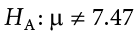
If the null hypothesis is rejected, then we will need some other explanation, which we call the alternative hypothesis, HA or H1. The alternative hypothesis is simply the reverse of the null hypothesis, and there are three options, depending on where we expect the difference to lie. Thus, our alternative hypothesis is the mathematical way of stating our research question. If we expect our obtained sample mean to be above or below the null hypothesis value, which we call a directional hypothesis, then our alternative hypothesis takes the form

based on the research question itself. We should only use a directional hypothesis if we have good reason, based on prior observations or research, to suspect a particular direction. When we do not know the direction, such as when we are entering a new area of research, we use a non-directional alternative:

We will set different criteria for rejecting the null hypothesis based on the directionality (greater than, less than, or not equal to) of the alternative. To understand why, we need to see where our criteria come from and how they relate to z scores and distributions.

Critical Values, p Values, and Significance Level

A low probability value casts doubt on the null hypothesis. How low must the probability value be in order to conclude that the null hypothesis is false? Although there is clearly no right or wrong answer to this question, it is conventional to conclude the null hypothesis is false if the probability value is less than .05. More conservative researchers conclude the null hypothesis is false only if the probability value is less than .01. When a researcher concludes that the null hypothesis is false, the researcher is said to have rejected the null hypothesis. The probability value below which the null hypothesis is rejected is called the level or simply (“alpha”). It is also called the significance level. If is not explicitly specified, assume that a = .05.

The significance level is a threshold we set before collecting data in order to determine whether or not we should reject the null hypothesis. We set this value beforehand to avoid biasing ourselves by viewing our results and then determining what criteria we should use. If our data produce values that meet or exceed this threshold, then we have sufficient evidence to reject the null hypothesis; if not, we fail to reject the null (we never “accept” the null).

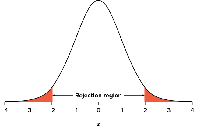
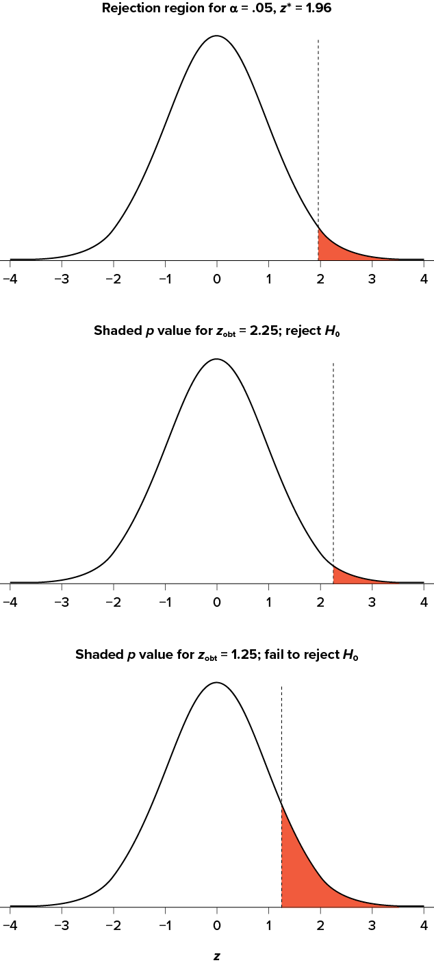
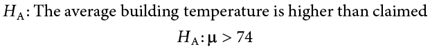
There are two criteria we use to assess whether our data meet the thresholds established by our chosen significance level, and they both have to do with our discussions of probability and distributions. Recall that probability refers to the likelihood of an event, given some situation or set of conditions. In hypothesis testing, that situation is the assumption that the null hypothesis value is the correct value, or that there is no effect. The value laid out in H0 is our condition under which we interpret our results. To reject this assumption, and thereby reject the null hypothesis, we need results that would be very unlikely if the null was true. Now recall that values of z which fall in the tails of the standard normal distribution represent unlikely values. That is, the proportion of the area under the curve as extreme as z—or more extreme than z—is very small as we get into the tails of the distribution. Our significance level corresponds to the area in the tail that is exactly equal to . If we use our normal criterion of a = .05, then 5% of the area under the curve becomes what we call the rejection region (also called the critical region) of the distribution. This is illustrated in Figure 7.1. The shaded rejection region takes us 5% of the area under the curve. Any result that falls in that region is sufficient evidence to reject the null hypothesis.

The rejection region is bounded by a specific z value, as is any area under the curve. In hypothesis testing, the value corresponding to a specific rejection region is called the critical value, zcrit (“z crit”), or z* (hence the other name “critical region”). Finding the critical value works exactly the same as finding the z score corresponding to any area under the curve as we did in Unit 1. If we go to the normal table, we will find that the z score corresponding to 5% of the area under the curve is equal to 1.645 (z = 1.64 corresponds to .0505 and z = 1.65 corresponds to .0495, so .05 is exactly in between them) if we go to the right and −1.645 if we go to the left. The direction must be determined by your alternative hypothesis, and drawing and shading the distribution is helpful for keeping directionality straight.

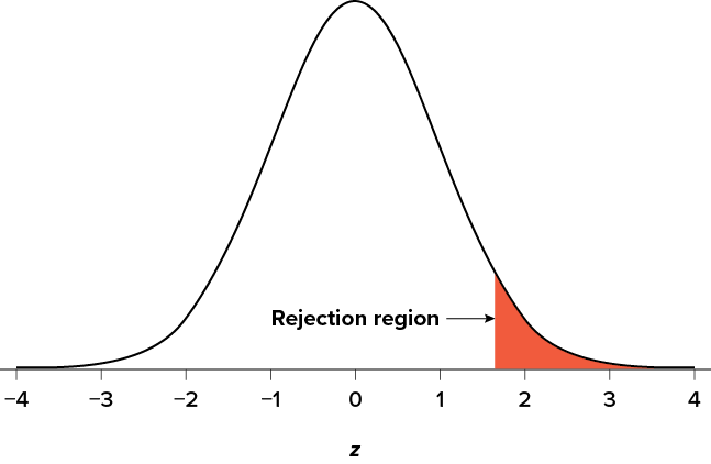
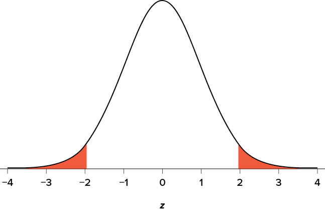
Suppose, however, that we want to do a non-directional test. We need to put the critical region in both tails, but we don’t want to increase the overall size of the rejection region (for reasons we will see later). To do this, we simply split it in half so that an equal proportion of the area under the curve falls in each tail’s rejection region. For a = .05, this means 2.5% of the area is in each tail, which, based on the z table, corresponds to critical values of z* = ±1.96. This is shown in Figure 7.2.

Thus, any z score falling outside ±1.96 (greater than 1.96 in absolute value) falls in the rejection region. When we use z scores in this way, the obtained value of z (sometimes called z obtained and abbreviated zobt) is something known as a test statistic, which is simply an inferential statistic used to test a null hypothesis. The formula for our z statistic has not changed:

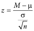
To formally test our hypothesis, we compare our obtained z statistic to our critical z value. If zobt > zcrit, that means it falls in the rejection region (to see why, draw a line for z = 2.5 on Figure 7.1 or Figure 7.2) and so we reject H0. If zobt < zcrit, we fail to reject. Remember that as z gets larger, the corresponding area under the curve beyond z gets smaller. Thus, the proportion, or p value, will be smaller than the area for , and if the area is smaller, the probability gets smaller. Specifically, the probability of obtaining that result, or a more extreme result, under the condition that the null hypothesis is true gets smaller.

The z statistic is very useful when we are doing our calculations by hand. However, when we use computer software, it will report to us a p value, which is simply the proportion of the area under the curve in the tails beyond our obtained z statistic. We can directly compare this p value to to test our null hypothesis: if p < a, we reject H0, but if p > a, we fail to reject. Note also that the reverse is always true. If we use critical values to test our hypothesis, we will always know if p is greater than or less than . If we reject, we know that p < a because the obtained z statistic falls farther out into the tail than the critical z value that corresponds to , so the proportion (p value) for that z statistic will be smaller. Conversely, if we fail to reject, we know that the proportion will be larger than because the z statistic will not be as far into the tail. This is illustrated for a one-tailed test in Figure 7.3.

When the null hypothesis is rejected, the effect is said to have statistical significance, or be statistically significant. For example, in the Physicians’ Reactions case study, the probability value is .0057. Therefore, the effect of obesity is statistically significant and the null hypothesis that obesity makes no difference is rejected. It is important to keep in mind that statistical significance means only that the null hypothesis of exactly no effect is rejected; it does not mean that the effect is important, which is what “significant” usually means. When an effect is significant, you can have confidence the effect is not exactly zero. Finding that an effect is significant does not tell you about how large or important the effect is.

Do not confuse statistical significance with practical significance. A small effect can be highly significant if the sample size is large enough.

Why does the word “significant” in the phrase “statistically significant” mean something so different from other uses of the word? Interestingly, this is because the meaning of “significant” in everyday language has changed. It turns out that when the procedures for hypothesis testing were developed, something was “significant” if it signified something. Thus, finding that an effect is statistically significant signifies that the effect is real and not due to chance. Over the years, the meaning of “significant” changed, leading to the potential misinterpretation.

The Hypothesis Testing Process

A Four-Step Procedure

The process of testing hypotheses follows a simple four-step procedure. This process will be what we use for the remainder of the textbook and course, and although the hypothesis and statistics we use will change, this process will not.

Step 1: State the Hypotheses

Your hypotheses are the first thing you need to lay out. Otherwise, there is nothing to test! You have to state the null hypothesis (which is what we test) and the alternative hypothesis (which is what we expect). These should be stated mathematically as they were presented above and in words, explaining in normal English what each one means in terms of the research question.

Step 2: Find the Critical Values

Next, we formally lay out the criteria we will use to test our hypotheses. There are two pieces of information that inform our critical values: , which determines how much of the area under the curve composes our rejection region, and the directionality of the test, which determines where the region will be.

Step 3: Calculate the Test Statistic and Effect Size

Once we have our hypotheses and the standards we use to test them, we can collect data and calculate our test statistic—in this case z. This step is where the vast majority of differences in future chapters will arise: different tests used for different data are calculated in different ways, but the way we use and interpret them remains the same. As part of this step, we will also calculate effect size to better quantify the magnitude of the difference between our groups. Although effect size is not considered part of hypothesis testing, reporting it as part of the results is approved convention.

Step 4: Make the Decision

Finally, once we have our obtained test statistic, we can compare it to our critical value and decide whether we should reject or fail to reject the null hypothesis. When we do this, we must interpret the decision in relation to our research question, stating what we concluded, what we based our conclusion on, and the specific statistics we obtained.

Example A Movie Popcorn

Let’s see how hypothesis testing works in action by working through an example. Say that a movie theater owner likes to keep a very close eye on how much popcorn goes into each bag sold, so he knows that the average bag has 8 cups of popcorn and that this varies a little bit, about half a cup. That is, the known population mean is = 8.00 and the known population standard deviation is s = 0.50. The owner wants to make sure that the newest employee is filling bags correctly, so over the course of a week he randomly assesses 25 bags filled by the employee to test for a difference (N = 25). He doesn’t want bags over-filled or under-filled, so he looks for differences in both directions. This scenario has all of the information we need to begin our hypothesis testing procedure.

Step 1: State the Hypotheses

Our manager is looking for a difference in the mean weight of popcorn bags compared to the population mean of 8. We will need both a null and an alternative hypothesis written both mathematically and in words. We’ll always start with the null hypothesis:

Notice that we phrase the hypothesis in terms of the population parameter , which in this case would be the true average weight of bags filled by the new employee. Our assumption of no difference, the null hypothesis, is that this mean is exactly the same as the known population mean value we want it to match, 8.00. Now let’s do the alternative:

In this case, we don’t know if the bags will be too full or not full enough, so we do a two-tailed alternative hypothesis that there is a difference.

Step 2: Find the Critical Values

Our critical values are based on two things: the directionality of the test and the level of significance. We decided in Step 1 that a two-tailed test is the appropriate directionality. We were given no information about the level of significance, so we assume that a = .05 is what we will use. As stated earlier in the chapter, the critical values for a two-tailed z test at a = .05 are z* = ±1.96. This will be the criteria we use to test our hypothesis. We can now draw out our distribution, as shown in Figure 7.4, so we can visualize the rejection region and make sure it makes sense.

Step 3: Calculate the Test Statistic and Effect Size

Now we come to our formal calculations. Let’s say that the manager collects data and finds that the average weight of this employee’s popcorn bags is M = 7.75 cups. We can now plug this value, along with the values presented in the original problem, into our equation for z:

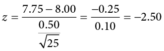
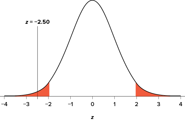
So our test statistic is z = −2.50, which we can draw onto our rejection region distribution as shown in Figure 7.5.

Effect Size

When we reject the null hypothesis, we are stating that the difference we found was statistically significant, but we have mentioned several times that this tells us nothing about practical significance. To get an idea of the actual size of what we found, we can compute a new statistic called an effect size. Effect size gives us an idea of how large, important, or meaningful a statistically significant effect is. For mean differences like we calculated here, our effect size is Cohen’s d:

This is very similar to our formula for z, but we no longer take into account the sample size (since overly large samples can make it too easy to reject the null). Cohen’s d is interpreted in units of standard deviations, just like z. For our example:

Cohen’s d is interpreted as small, moderate, or large. Specifically, d = 0.20 is small, d = 0.50 is moderate, and d = 0.80 is large. Obviously, values can fall in between these guidelines, so we should use our best judgment and the context of the problem to make our final interpretation of size. Our effect size happens to be exactly equal to one of these, so we say that there is a moderate effect.

Effect sizes are incredibly useful and provide important information and clarification that overcomes some of the weakness of hypothesis testing. Any time you perform a hypothesis test, whether statistically significant or not, you should always calculate and report effect size.

Step 4: Make the Decision

Looking at Figure 7.5, we can see that our obtained z statistic falls in the rejection region. We can also directly compare it to our critical value: in terms of absolute value, −2.50 > −1.96, so we reject the null hypothesis. We can now write our conclusion:

Reject H0. Based on the sample of 25 bags, we can conclude that the average popcorn bag from this employee is smaller (M = 7.75 cups) than the average weight of popcorn bags at this movie theater, and the effect size was moderate, z = −2.50, p < .05, d = 0.50.

When we write our conclusion, we write out the words to communicate what it actually means, but we also include the average sample size we calculated (the exact location doesn’t matter, just somewhere that flows naturally and makes sense), the z statistic and p value, and the effect size. We don’t know the exact p value, but we do know that because we rejected the null, it must be less than .

Example B Office Temperature

Let’s do another example to solidify our understanding. Let’s say that the office building you work in is supposed to be kept at 74 degrees Fahrenheit during the summer months but is allowed to vary by 1 degree in either direction. You suspect that, as a cost saving measure, the temperature was secretly set higher. You set up a formal way to test your hypothesis.

Step 1: State the Hypotheses

You start by laying out the null hypothesis:

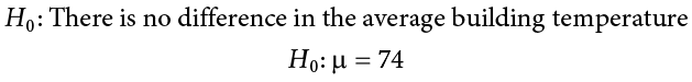
Next you state the alternative hypothesis. You have reason to suspect a specific direction of change, so you make a one-tailed test:

Step 2: Find the Critical Values

You know that the most common level of significance is a = .05, so you keep that the same and know that the critical value for a one-tailed z test is z* = 1.645. To keep track of the directionality of the test and rejection region, you draw out your distribution as shown in Figure 7.6.

Step 3: Calculate the Test Statistic and Effect Size

Now that you have everything set up, you spend one week collecting temperature data:

You calculate the average of these scores to be M = 76.6 degrees. You use this to calculate the test statistic, using = 74 (the supposed average temperature), s = 1.00 (how much the temperature should vary), and n = 5 (how many data points you collected):

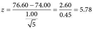
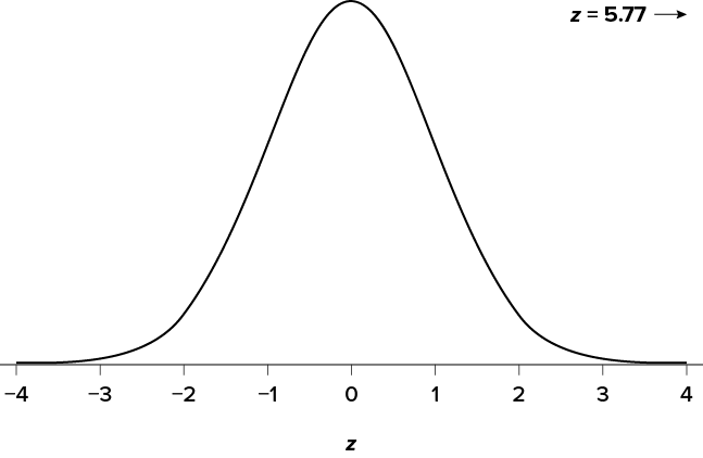
This value falls so far into the tail that it cannot even be plotted on the distribution (Figure 7.7)! Because the result is significant, you also calculate an effect size:

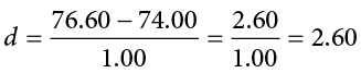
The effect size you calculate is definitely large, meaning someone has some explaining to do!

Step 4: Make the Decision

You compare your obtained z statistic, z = 5.77, to the critical value, z* = 1.645, and find that z > z*. Therefore you reject the null hypothesis, concluding:

Reject H0. Based on 5 observations, the average temperature (M = 76.6 degrees) is statistically significantly higher than it is supposed to be, and the effect size was large, z = 5.77, p < .05, d = 2.60.

Example C Different Significance Level

Finally, let’s take a look at an example phrased in generic terms, rather than in the context of a specific research question, to see the individual pieces one more time. This time, however, we will use a stricter significance level, a = .01, to test the hypothesis.

Step 1: State the Hypotheses

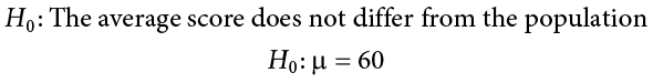
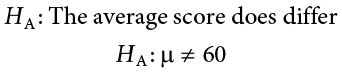
We will use 60 as an arbitrary null hypothesis value:

We will assume a two-tailed test:

Step 2: Find the Critical Values

We have seen the critical values for z tests at a = .05 levels of significance several times. To find the values for a = .01, we will go to the Standard Normal Distribution Table and find the z score cutting off .005 (.01 divided by 2 for a two-tailed test) of the area in the tail, which is z* = ±2.575. Notice that this cutoff is much higher than it was for a = .05. This is because we need much less of the area in the tail, so we need to go very far out to find the cutoff. As a result, this will require a much larger effect or much larger sample size in order to reject the null hypothesis.

Step 3: Calculate the Test Statistic and Effect Size

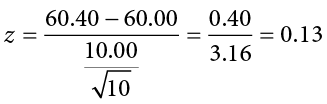
We can now calculate our test statistic. We will use s = 10 as our known population standard deviation and the following data to calculate our sample mean:

The average of these scores is M = 60.40. From this we calculate our z statistic as:

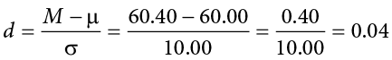
The Cohen’s d effect size calculation is:

Step 4: Make the Decision

Our obtained z statistic, z = 0.13, is very small. It is much less than our critical value of 2.575. Thus, this time, we fail to reject the null hypothesis. Our conclusion would look something like:

Fail to reject H0. Based on the sample of 10 scores, we cannot conclude that there is an effect causing the mean (M = 60.40) to be statistically significantly different from 60.00, z = 0.13, p > .01, d = 0.04, and the effect size supports this interpretation.

Notice two things about the end of the conclusion. First, we wrote that p is greater than instead of p is less than, like we did in the previous two examples. This is because we failed to reject the null hypothesis. We don’t know exactly what the p value is, but we know it must be larger than the level we used to test our hypothesis. Second, we used .01 instead of the usual .05, because this time we tested at a different level. The number you compare to the p value should always be the significance level you test at.

Other Considerations in Hypothesis Testing

There are several other considerations we need to keep in mind when performing hypothesis testing.

Errors in Hypothesis Testing

In the Physicians’ Reactions case study, the probability value associated with the significance test is .0057. Therefore, the null hypothesis was rejected, and it was concluded that physicians intend to spend less time with obese patients. Despite the low probability value, it is possible that the null hypothesis of no true difference between obese and average-weight patients is true and that the large difference between sample means occurred by chance. If this is the case, then the conclusion that physicians intend to spend less time with obese patients is in error. This type of error is called a Type I error. More generally, a Type I error occurs when a significance test results in the rejection of a true null hypothesis.

By one common convention, if the probability value is below .05, then the null hypothesis is rejected. Another convention, although slightly less common, is to reject the null hypothesis if the probability value is below .01. The threshold for rejecting the null hypothesis is called the level or simply . It is also called the significance level. As discussed in the introduction to hypothesis testing, it is better to interpret the probability value as an indication of the weight of evidence against the null hypothesis than as part of a decision rule for making a reject or do-not-reject decision. Therefore, keep in mind that rejecting the null hypothesis is not an all-or-nothing decision.

The Type I error rate is affected by the level: the lower the level the lower the Type I error rate. It might seem that is the probability of a Type I error. However, this is not correct. Instead, is the probability of a Type I error given that the null hypothesis is true. If the null hypothesis is false, then it is impossible to make a Type I error.

The second type of error that can be made in significance testing is failing to reject a false null hypothesis. This kind of error is called a Type II error. Unlike a Type I error, a Type II error is not really an error. When a statistical test is not significant, it means that the data do not provide strong evidence that the null hypothesis is false. Lack of significance does not support the conclusion that the null hypothesis is true. Therefore, a researcher should not make the mistake of incorrectly concluding that the null hypothesis is true when a statistical test was not significant. Instead, the researcher should consider the test inconclusive. Contrast this with a Type I error in which the researcher erroneously concludes that the null hypothesis is false when, in fact, it is true.

A Type II error can only occur if the null hypothesis is false. If the null hypothesis is false, then the probability of a Type II error is called b (“beta”). The probability of correctly rejecting a false null hypothesis equals 1 − b and is called statistical power. Power is simply our ability to correctly detect an effect that exists. It is influenced by the size of the effect (larger effects are easier to detect), the significance level we set (making it easier to reject the null makes it easier to detect an effect, but increases the likelihood of a Type I error), and the sample size used (larger samples make it easier to reject the null).

Misconceptions in Hypothesis Testing

Misconceptions about significance testing are common. This section lists three important ones.

1. Misconception: The probability value (p value) is the probability that the null hypothesis is false.
   Proper interpretation: The probability value (p value) is the probability of a result as extreme or more extreme given that the null hypothesis is true. It is the probability of the data given the null hypothesis. It is not the probability that the null hypothesis is false.
2. Misconception: A low probability value indicates a large effect.
   Proper interpretation: A low probability value indicates that the sample outcome (or an outcome more extreme) would be very unlikely if the null hypothesis were true. A low probability value can occur with small effect sizes, particularly if the sample size is large.
3. Misconception: A non-significant outcome means that the null hypothesis is probably true.
   Proper interpretation: A non-significant outcome means that the data do not conclusively demonstrate that the null hypothesis is false.

Exercises

1. In your own words, explain what the null hypothesis is.
2. What are Type I and Type II errors?
3. What is ?
4. Why do we phrase null and alternative hypotheses with population parameters and not sample means?
5. If our null hypothesis is “H0 : = 40,” what are the three possible alternative hypotheses?
6. Why do we state our hypotheses and decision criteria before we collect our data?
7. Why do you calculate an effect size?
8. Determine whether you would reject or fail to reject the null hypothesis in the following situations:
   1. z = 1.99, two-tailed test at a = .05
   2. z = 0.34, z* = 1.645
   3. p = .03, a = .05
   4. p = .015, a = .01
9. You are part of a trivia team and have tracked your team’s performance since you started playing, so you know that your scores are normally distributed with = 78 and s = 12. Recently, a new person joined the team, and you think the scores have gotten better. Use hypothesis testing to see if the average score has improved based on 9 weeks’ worth of score data where is 88.75.
10. You get hired as a server at a local restaurant, and the manager tells you that servers’ tips are $42 on average but vary about $12 ( = 42, s = 12). You decide to track your tips to see if you make a different amount, but because this is your first job as a server, you don’t know if you will make more or less in tips. After working 16 shifts, you find that your average nightly amount is $44.50 from tips. Test for a difference between this value and the population mean at the a = .05 level of significance.

“Null Hypothesis” by Randall Munroe/xkcd.com is licensed under CC BY-NC 2.5.)