9 Chapter 9: Related Samples

So far, we have dealt with data measured on a single variable at a single point in time, allowing us to gain an understanding of the logic and process behind statistics and hypothesis testing. Now, we will look at a slightly different type of data that has new information we couldn’t get at before: change. Specifically, we will look at how the value of a variable, within people, changes across two time points. This is a very powerful thing to do, and, as we will see shortly, it involves only a very slight addition to our existing process and does not change the mechanics of hypothesis testing or formulas at all!

Change and Differences

Researchers are often interested in change over time. Sometimes we want to see if change occurs naturally, and other times we are hoping for change in response to some manipulation. In each of these cases, we measure a single variable at different times, and what we are looking for is whether or not we get the same score at Time 2 as we did at Time 1. The absolute value of our measurements does not matter—all that matters is the change, or the difference score. Let’s look at an example.

Table 9.1 shows scores on a quiz that five employees received before they took a training course and after they took the course. The difference between these scores (i.e., the score after minus the score before) represents improvement in the employees’ ability. The third column is what we look at when assessing whether our training was effective. We want to see positive scores, which indicate that the employees’ performance went up. What we are not interested in is how good they were before the training or after the training. Notice that the lowest-scoring employee before the training (with a score of 1) improved just as much as the highest scoring employee before the training (with a score of 8), regardless of how far apart they were to begin with. There’s also one improvement score of 0, meaning that the training did not help this employee. An important factor in this is that the participants received the same assessment at both time points. To calculate improvement or any other difference score, we must measure only a single variable.

When looking at change scores like the ones in Table 9.1, we calculate our difference scores by taking the Time 2 score and subtracting the Time 1 score. That is:

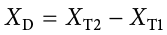
Where XD is the difference score, XT1 is the score on the variable at Time 1, and XT2 is the score on the variable at Time 2. The difference score, XD, will be the data we use to test for improvement or change. We subtract Time 2 minus Time 1 for ease of interpretation; if scores get better, then the difference score will be positive. Similarly, if we’re measuring something like reaction time or depression symptoms that we are trying to reduce, then better outcomes (lower scores) will yield negative difference scores.

While we frequently use difference scores for data that are collected from the same participants twice, we can also test to see if people who are matched or paired in some way agree on a specific topic. These are called matched pairs data. For example, we can see if a parent and a child agree on the quality of home life, or we can see if two romantic partners agree on how serious and committed their relationship is. In these situations, we also subtract one score from the other to get a difference score. This time, however, it doesn’t matter which score we subtract from the other because what we are concerned with is the agreement.

In both of these types of data, what we have are multiple scores on a single variable. That is, a single observation or data point is comprised of two measurements that are put together into one difference score. This is what makes the analysis of change unique—our ability to link these measurements in a meaningful way. This type of analysis would not work if we had two separate samples of people that weren’t related at the individual level, such as samples of people from different states that we gathered independently. Such datasets and analyses are the subject of Chapter 10.

A Rose by Any Other Name . . .

It is important to point out that the related samples t test has been called many different things by many different people over the years: related samples, paired samples, matched pairs, repeated measures, dependent measures, dependent samples, and many others. What all of these names have in common is that they describe the analysis of two scores that are related in a systematic way within people or within pairs, which is what each of the datasets usable in this analysis have in common. As such, all of these names are equally appropriate, and the choice of which one to use comes down to preference. In this text, we will refer to related samples, though the appearance of any of the other names throughout this chapter should not be taken to refer to a different analysis; they are all the same thing.

Now that we have an understanding of what difference scores are and know how to calculate them, we can use them to test hypotheses. As we will see, this works exactly the same way as testing hypotheses about one sample mean with a t statistic. The only difference is in the format of the null and alternative hypotheses.

Hypotheses of Change and Differences

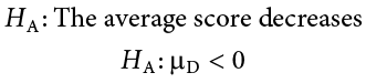
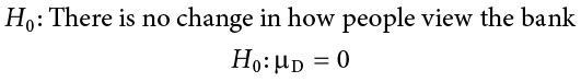
When we work with difference scores, our research questions have to do with change. Did scores improve? Did symptoms get better? Did prevalence go up or down? Our hypotheses will reflect this. Remember that the null hypothesis is the idea that there is nothing interesting, notable, or impactful represented in our dataset. In a related samples t test, that takes the form of “no change.” There is no improvement in scores or decrease in symptoms. Thus, our null hypothesis is:

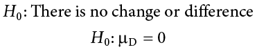
As with our other null hypotheses, we express the null hypothesis for related samples t tests in both words and mathematical notation. The exact wording of the written-out version should be changed to match whatever research question we are addressing (e.g., “There is no change in ability scores after training”). However, the mathematical version of the null hypothesis is always exactly the same: the average change score is equal to zero. Our population parameter for the average is still , but it now has a subscript D to denote the fact that it is the average change score and not the average raw observation before or after our manipulation. Obviously, individual difference scores can go up or down, but the null hypothesis states that these positive or negative change values are just random chance and that the true average change score across all people is 0.

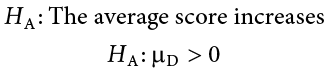
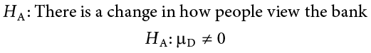
Our alternative hypotheses will also follow the same format that they did before: they can be directional if we suspect a change or difference in a specific direction, or we can use an inequality sign to test for any change:

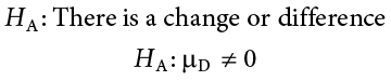
As before, your choice of which alternative hypothesis to use should be specified before you collect data based on your research question and any evidence you might have that would indicate a specific directional (or non-directional) change.

Critical Values and Decision Criteria

As with before, once we have our hypotheses laid out, we need to find the critical values that will serve as our decision criteria. This step has not changed at all from Chapter 8. Our critical values are based on our level of significance (still usually a = .05), the directionality of our test (one-tailed or two-tailed), and the degrees of freedom, which are still calculated as df = n − 1. Because this is a t test like the last chapter, we will find our critical values on the same t table using the same process of identifying the correct column based on our significance level and directionality and the correct row based on our degrees of freedom or the next lowest value if our exact degrees of freedom are not presented. After we calculate our test statistic, our decision criteria are the same as well: p < a or tobt > t*.

Test Statistic

Our test statistic for our change scores follows exactly the same format as it did for our one-sample t test. In fact, the only difference is in the data that we use. For our change test, we first calculate a difference score as shown above. Then, we use those scores as the raw data in the same mean calculation, standard error formula, and t statistic. Let’s look at each of these.

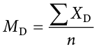
The mean difference score is calculated in the same way as any other mean: sum each of the individual difference scores and divide by the sample size.

Here we are using the subscript D to keep track of that fact that these are difference scores instead of raw scores; it has no actual effect on our calculation. Using this, we calculate the standard deviation of the difference scores the same way as well:

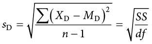
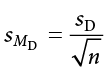
We will find the numerator, the sum of squares, using the same table format that we learned in Chapter 3. Once we have our standard deviation, we can find the standard error:

Finally, our test statistic t has the same structure as well:

As we can see, once we calculate our difference scores from our raw measurements, everything else is exactly the same. Let’s see an example.

Example A Increasing Satisfaction at Work

Workers at a local company have been complaining that working conditions have gotten very poor, hours are too long, and they don’t feel supported by the management. The company hires a consultant to come in and help fix the situation before it gets so bad that the employees start to quit. The consultant first assesses 40 of the employees’ level of job satisfaction as part of focus groups used to identify specific changes that might help. The company institutes some of these changes, and six months later the consultant returns to measure job satisfaction again. Knowing that some interventions miss the mark and can actually make things worse, the consultant tests for a difference in either direction (i.e., and increase or a decrease in average job satisfaction) at the a = .05 level of significance.

Step 1: State the Hypotheses

First, we state our null and alternative hypotheses:

In this case, we are hoping that the changes we made will improve employee satisfaction, and, because we based the changes on employee recommendations, we have good reason to believe that they will. Thus, we will use a one-directional alternative hypothesis.

Step 2: Find the Critical Values

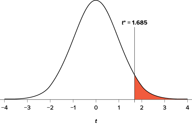
Our critical values will once again be based on our level of significance, which we know is a = .05, the directionality of our test, which is one-tailed to the right, and our degrees of freedom. For our related-samples t test, the degrees of freedom are still given as df = n − 1. For this problem, we have 40 people, so our degrees of freedom are 39. Going to our t table, we find that the critical value is t* = 1.685 as shown in Figure 9.1.

Step 3: Calculate the Test Statistic and Effect Size

Now that the criteria are set, it is time to calculate the test statistic. The data obtained by the consultant found that the difference scores from Time 1 to Time 2 had a mean of = 2.96 and a standard deviation of sD = 2.85. Using this information, plus the size of the sample (n = 40), we first calculate the standard error:

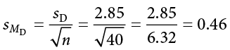
Now, we can put that value, along with our sample mean and null hypothesis value, into the formula for t and calculate the test statistic:

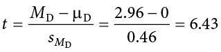
Notice that, because the null hypothesis value of a related samples t test is always 0, we can simply divide our obtained sample mean by the standard error.

Next, we will calculate Cohen’s d as an effect size using the same format as we did for the last t test:

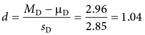
This is a large effect size. Notice again that we can omit the null hypothesis value here because it is always equal to 0.

Step 4: Make the Decision

We have obtained a test statistic of t = 6.43 that we can compare to our previously established critical value of t* = 1.685. The number 6.43 is larger than 1.685, so t > t* and we reject the null hypothesis:

Reject H0. Based on the sample data from 40 workers, we can say that the intervention statistically significantly improved job satisfaction ( = 2.96, SDD = 2.85) among the workers, t(39) = 6.43, p < .05, d = 1.04.

Hopefully, the above example made it clear that running a related samples t test to look for differences before and after some treatment works exactly the same way as a regular one-sample t test does, which was just a small change in how z tests were performed in Chapter 7. At this point, this process should feel familiar, and we will continue to make small adjustments to this familiar process as we encounter new types of data to test new types of research questions.

Example B Bad Press

Let’s say that a bank wants to make sure that their new commercial will make them look good to the public, so they recruit 7 people to view the commercial as a focus group. The focus group members fill out a short questionnaire about how they view the company, then watch the commercial and fill out the same questionnaire a second time. The bank really wants to find significant results, so they test for a change at a = .10. However, they use a two-tailed test since they know that past commercials have not gone over well with the public, and they want to make sure the new one does not backfire. They decide to test their hypothesis using a confidence interval to see just how spread-out the opinions are. As we will see, confidence intervals work the same way as they did before, just like with the test statistic.

Step 1: State the Hypotheses

As always, we start with hypotheses:

Step 2: Find the Critical Values

Just like with our regular hypothesis testing procedure, we will need critical values from the appropriate level of significance and degrees of freedom in order to form our confidence interval. Because we have 7 participants, our degrees of freedom are df = 6. From our t table, we find that the critical value corresponding to this df at this level of significance is t* = 1.943.

Step 3: Calculate the Confidence Interval

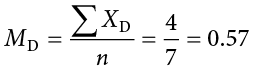
The data collected before (Time 1) and after (Time 2) the participants viewed the commercial is presented in Table 9.2. In order to build our confidence interval, we will first have to calculate the mean and standard deviation of the difference scores, which are also in Table 9.2. As a reminder, the difference scores are calculated as Time 2 − Time 1.

The mean of the difference scores is:

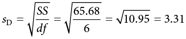
The standard deviation will be solved by first using the sum of squares table:

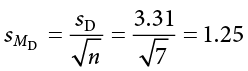
Finally, we find the standard error:

We now have all the pieces needed to compute our confidence interval:

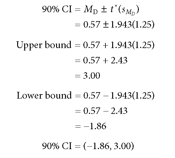
Step 4: Make the Decision

Remember that the confidence interval represents a range of values that seem plausible or reasonable based on our observed data. The interval spans −1.86 to 3.00, which includes 0, our null hypothesis value. Because the null hypothesis value is in the interval, it is considered a reasonable value, and because it is a reasonable value, we have no evidence against it. We fail to reject the null hypothesis.

Fail to reject H0. Based on our focus group of 7 people, we cannot say that the average change in opinion ( = 0.57, SDD = 3.31) was any better or worse after viewing the commercial, 90% CI: (−1.86, 3.00).

As with before, we only report the confidence interval to indicate how we performed the test.

Exercises

1. What is the difference between a one-sample t test and a related-samples t test? How are they alike?
2. Name three research questions that could be addressed using a related-samples t test.
3. What are difference scores and why do we calculate them?
4. Why is the null hypothesis for a related-samples t test always D = 0?
5. A researcher is interested in testing whether explaining the processes of statistics helps increase trust in computer algorithms. He wants to test for a difference at the a = .05 level and knows that some people may trust the algorithms less after the training, so he uses a two-tailed test. He gathers pre-post data from 35 people and finds that the average difference score is = 12.10 with a standard deviation of sD = 17.39. Conduct a hypothesis test to answer the research question.
6. Decide whether you would reject or fail to reject the null hypothesis in the following situations:
   1. = 3.50, sD = 1.10, n = 12, a = .05, two-tailed test
   2. 95% CI = (0.20, 1.85)
   3. t = 2.98, t* = −2.36, one-tailed test to the left
   4. 90% CI = (−1.12, 4.36)
7. Calculate difference scores for the following data:
   

   Time 1	Time 2	XD
   61	83
   75	89
   91	98
   83	92
   74	80
   82	88
   98	98
   82	77
   69	88
   76	79
   91	91
   70	80

8. Researchers investigated the extent to which Japanese immigrant mothers encouraged their infants to interact with them or with objects in their environment (such as toys). The researchers observed 8 mothers with their infants. Data are the number of times that mothers encouraged their infants to engage with them or with objects during the observation period. Test the hypothesis at the a = .05 level using the four-step hypothesis testing procedure.
   

   With Mom	With Objects
   15	40
   12	47
   14	32
   10	50
   20	35
   28	45
   12	42
   15	32

9. Construct confidence intervals from a mean of = 1.25, standard error of = 0.45, and df = 10 at the 90%, 95%, and 99% confidence levels. Describe what happens as confidence changes and whether to reject H0.
10. A professor wants to see how much students learn over the course of a semester. A pre-test is given before the class begins to see what students know ahead of time, and the same test is given at the end of the semester to see what students know at the end. The data are below. Test for an improvement at the a = .05 level. Did scores increase? How much did scores increase?
    

    Pre-test	Post-test	XD
    90	89
    60	66
    95	99
    93	91
    95	100
    67	64
    89	91
    90	95
    94	95
    83	89
    75	82
    87	92
    82	83
    82	85
    88	93
    66	69
    90	90
    93	100
    86	95
    91	96