11 Chapter 11: Analysis of Variance
Analysis of variance (ANOVA) serves the same purpose as the t tests we learned in Unit 2: it tests for differences in group means. ANOVA is more flexible in that it can handle any number of groups, unlike t tests, which are limited to two groups (independent samples) or two time points (dependent samples). Thus, the purpose and interpretation of ANOVA will be the same as it was for t tests, as will the hypothesis-testing procedure. However, ANOVA will, at first glance, look much different from a mathematical perspective, although as we will see, the basic logic behind the test statistic for ANOVA is actually the same. This chapter will describe the general design of ANOVA, with a focus on calculating the independent samples one-way ANOVA, which is an extension of the independent samples t test, where three or more different groups are compared on a single independent (or grouping) variable.
Observing and Interpreting Variability
We have seen time and again that scores, be they individual data or group means, will differ naturally. Sometimes this is due to random chance, and other times it is due to actual differences. Our job as scientists, researchers, and data analysts is to determine if the observed differences are systematic and meaningful (via a hypothesis test) and, if so, what is causing those differences. Through this, it becomes clear that, although we are usually interested in the mean or average score, it is the variability in the scores that is key.
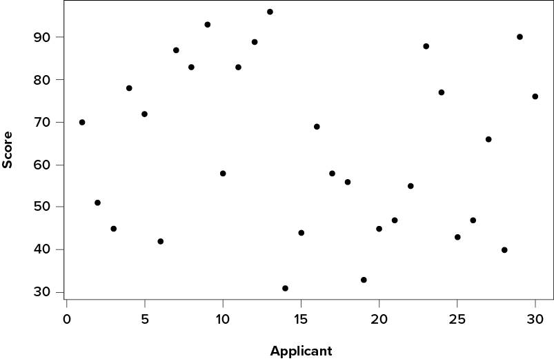
Take a look at Figure 11.1, which shows scores for many people on a test of skill used as part of a job application. The x-axis has each individual person, in no particular order, and the y-axis contains the score each person received on the test. As we can see, the job applicants differed quite a bit in their performance, and understanding why that is the case would be extremely useful information. However, there’s no interpretable pattern in the data, especially because we only have information on the test, not on any other variable (remember that the x-axis here only shows individual people and is not ordered or interpretable).
Figure 11.1. Scores on a job test. (“Job Test Scores” by Judy Schmitt is licensed under CC BY-NC-SA 4.0.)
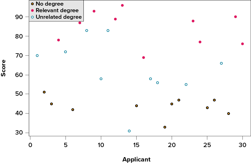
Our goal is to explain this variability that we are seeing in the dataset. Let’s assume that as part of the job application procedure we also collected data on the highest degree each applicant earned. With knowledge of what the job requires, we could sort our applicants into three groups: applicants who have a college degree related to the job, applicants who have a college degree that is not related to the job, and applicants who did not earn a college degree. This is a common way that job applicants are sorted, and we can use ANOVA to test if these groups are actually different. Figure 11.2 presents the same job applicant scores, but now they are color coded by group membership (i.e., which group they belong in). Now that we can differentiate between applicants this way, a pattern starts to emerge: applicants with a relevant degree (coded red) tend to be near the top, applicants with no college degree (coded black) tend to be near the bottom, and applicants with an unrelated degree (coded green) tend to fall into the middle. However, even within these groups, there is still some variability, as shown in Figure 11.2.
Figure 11.2. Applicant scores coded by degree earned. (“Job Test Scores by Degree” by Judy Schmitt is licensed under CC BY-NC-SA 4.0.)
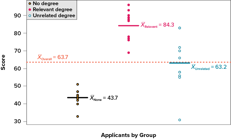
This pattern is even easier to see when the applicants are sorted and organized into their respective groups, as shown in Figure 11.3.
Figure 11.3. Applicant scores by group. (“Job Test Scores by Group” by Judy Schmitt is licensed under CC BY-NC-SA 4.0.)
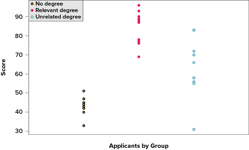
Now that we have our data visualized into an easily interpretable format, we can clearly see that our applicants’ scores differ largely along group lines. Those applicants who do not have a college degree received the lowest scores, those who had a degree relevant to the job received the highest scores, and those who did have a degree but one that is not related to the job tended to fall somewhere in the middle. Thus, we have systematic variability between our groups.
We can also clearly see that within each group, our applicants’ scores differed from one another. Those applicants without a degree tended to score very similarly, since the scores are clustered close together. Our group of applicants with relevant degrees varied a little bit more than that, and our group of applicants with unrelated degrees varied quite a bit. It may be that there are other factors that cause the observed score differences within each group, or they could just be due to random chance. Because we do not have any other explanatory data in our dataset, the variability we observe within our groups is considered random error, with any deviations between a person and that person’s group mean caused only by chance. Thus, we have unsystematic (random) variability within our groups.
The process and analyses used in ANOVA will take these two sources of variability (systematic variability between groups and random error within groups, or how much groups differ from each other and how much people differ within each group) and compare them to one another to determine if the groups have any explanatory value in our outcome variable. By doing this, we will test for statistically significant differences between the group means, just like we did for t tests. We will go step by step to break down the math to see how ANOVA actually works.
Sources of Variability
ANOVA is all about looking at the different sources of variability (i.e., the reasons that scores differ from one another) in a dataset. Fortunately, the way we calculate these sources of variability takes a very familiar form: the sum of squares. Before we get into the calculations themselves, we must first lay out some important terminology and notation.
In ANOVA, we are working with two variables, a grouping or explanatory variable and a continuous outcome variable. The grouping variable is our predictor (it predicts or explains the values in the outcome variable) or, in experimental terms, our independent variable, and is made up of k groups, with k being any whole number 2 or greater. That is, ANOVA requires two or more groups to work, and it is usually conducted with three or more. In ANOVA, we refer to groups as levels, so the number of levels is just the number of groups, which again is k. In the above example, our grouping variable was education, which had 3 levels, so k = 3. When we report any descriptive value (e.g., mean, sample size, standard deviation) for a specific group, we will use a subscript 1…k to denote which group it refers to. For example, if we have three groups and want to report the standard deviation s for each group, we would report them as s1, s2, and s3.
Our second variable is our outcome variable. This is the variable on which people differ, and we are trying to explain or account for those differences based on group membership. In the example above, our outcome was the score each person earned on the test. Our outcome variable will still use X for scores as before. When describing the outcome variable using means, we will use subscripts to refer to specific, individual group means. So if we have k = 3 groups, our means will be  ,
,  , and
, and  . We will also have a single mean representing the average of all participants across all groups. This is known as the grand mean, and we use the symbol
  . These different means—the individual group means and the overall grand mean—will be how we calculate our sums of squares.
Finally, we now have to differentiate between several different sample sizes. Our data will now have sample sizes for each group, and we will denote these with a lower case n and a subscript, just like with our other descriptive statistics: n1, n2, and n3. We also have the overall sample size in our dataset, and we will denote this with a capital N. The total sample size is just the group sample sizes added together.
Between-Groups Sum of Squares
One source of variability we identified in Figure 11.3 of the above example was differences or variability between the groups. That is, the groups clearly had different average levels. The variability arising from these differences is known as between-groups variability, and between-groups sum of squares is used to calculate between-groups variability.
Our calculations for sums of squares in ANOVA will take on the same form as it did for regular calculations of variance. Each observation, in this case the group means, is compared to the overall mean, in this case the grand mean, to calculate a deviation score. These deviation scores are squared so that they do not cancel each other out and sum to zero. The squared deviations are then added up, or summed. There is, however, one small difference. Because each group mean represents a group composed of multiple people, before we sum the deviation scores we must multiply them by the number of people within that group. Incorporating this, we find our equation for between-groups sum of squares to be:
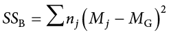
The subscript j refers to the “jth” group where j = 1…k to keep track of which group mean and sample size we are working with. As you can see, the only difference between this equation and the familiar sum of squares for variance is that we are adding in the sample size. Everything else logically fits together in the same way.
Within-Groups Sum of Squares
The other source of variability in the figures—within-groups variability—comes from differences that occur within each group. That is, each individual deviates a little bit from their respective group mean, just like the group means differed from the grand mean. We therefore label this source the within-groups variance. Because we are trying to account for variance based on group-level means, any deviation from the group means indicates an inaccuracy or error. Thus, our within-groups variability represents our error in ANOVA.
The formula for this sum of squares is again going to take on the same form and logic. What we are looking for is the distance between each individual person and the mean of the group to which they belong. We calculate this deviation score, square it so that they can be added together, then sum all of them into one overall value:
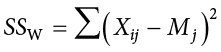
In this instance, because we are calculating this deviation score for each individual person, there is no need to multiple by how many people we have. The subscript j again represents a group and the subscript i refers to a specific person. So, Xij is read as “the ith person of the jth group.” It is important to remember that the deviation score for each person is only calculated relative to their group mean; do not calculate these scores relative to the other group means.
Total Sum of Squares
Total sum of squares can also be computed as a check for our calculations of between-groups and within-groups sums of squares. The calculation for this score is exactly the same as it would be if we were calculating the overall variance in the dataset (because that’s what we are interested in explaining) without worrying about or even knowing about the groups into which our scores fall:
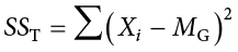
We can see that our total sum of squares is just each individual score minus the grand mean. As with our within-groups sum of squares, we are calculating a deviation score for each individual person, so we do not need to multiply anything by the sample size; that is only done for a between-groups sum of squares.
An important feature of the sums of squares in ANOVA is that they all fit together. We could work through the algebra to demonstrate that if we added together the formulas for SSB and SSW, we would end up with the formula for SST. That is:
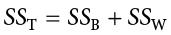
This will prove to be very convenient, because if we know the values of any two of our sums of squares, it is very quick and easy to find the value of the third. It is also a good way to check calculations: if you calculate each SS by hand, you can make sure that they all fit together as shown above, and if not, you know that you made a math mistake somewhere.
We can see from the above formulas that calculating an ANOVA by hand from raw data can take a very, very long time. For this reason, you will not be required to calculate the SS values by hand, but you should still take the time to understand how they fit together and what each one represents to ensure you understand the analysis itself.
ANOVA Table
All of our sources of variability fit together in meaningful, interpretable ways as we saw above, and the easiest way to show these relationships is to organize them in a table. The ANOVA table (Table 11.1) shows how we calculate the df, MS, and F values. The first column of the ANOVA table, labeled “Source,” indicates which of our sources of variability we are using: between groups (B), within groups (W), or total (T). The second column, labeled “SS,” contains our values for the sum of squared deviations, also known as the sum of squares, that we learned to calculate above.


As noted previously, calculating these by hand takes too long, so the formulas are not presented in Table 11.1. However, remember that SST is the sum of SSB and SSW, in case you are only given two SS values and need to calculate the third.
The next column, labeled “df,” is our degrees of freedom. As with the sums of squares, there is a different df for each group, and the formulas are presented in the table. Total degrees of freedom is calculated by subtracting 1 from the overall sample size (N). (Remember, the capital N in the df calculations refers to the overall sample size, not a specific group sample size.) Notice that dfT, just like for total sums of squares, is the Between (dfB) and Within (dfW) rows added together. If you take N − k + k − 1, then the “− k” and “+ k” portions will cancel out, and you are left with N − 1. This is a convenient way to quickly check your calculations.
The third column, labeled “MS,” shows our mean squared deviation for each source of variance. A mean square is just another way to say variability and is calculated by dividing the sum of squares by its corresponding degrees of freedom. Notice that we show this in the ANOVA table for the Between row and the Within row, but not for the Total row. There are two reasons for this. First, our Total mean square would just be the variance in the full dataset (put together the formulas to see this for yourself), so it would not be new information. Second, the mean square values for Between and Within would not add up to equal the Total mean square because they are divided by different denominators. This is in contrast to the first two columns, where the Total row was both the conceptual total (i.e., the overall variance and degrees of freedom) and the literal total of the other two rows.
The final column in the ANOVA table, labeled “F,” is our test statistic for ANOVA. The F statistic, just like a t or z statistic, is compared to a critical value to see whether we can reject for fail to reject a null hypothesis. Thus, although the calculations look different for ANOVA, we are still doing the same thing that we did in all of Unit 2. We are simply using a new type of data to test our hypotheses. We will see what these hypotheses look like shortly, but first, we must take a moment to address why we are doing our calculations this way.
ANOVA and Type I Error
You may be wondering why we do not just use another t test to test our hypotheses about three or more groups the way we did in Unit 2. After all, we are still just looking at group mean differences. The reason is that our t statistic formula can only handle up to two groups, one minus the other. With only two groups, we can move our population parameters for the group means around in our null hypothesis and still get the same interpretation: the means are equal, which can also be concluded if one mean minus the other mean is equal to zero. However, if we tried adding a third mean, we would no longer be able to do this. So, in order to use t tests to compare three or more means, we would have to run a series of individual group comparisons.
For only three groups, we would have three t tests: Group 1 vs. Group 2, Group 1 vs. Group 3, and Group 2 vs. Group 3. This may not sound like a lot, especially with the advances in technology that have made running an analysis very fast, but it quickly scales up. With just one additional group, bringing our total to four, we would have six comparisons: Group 1 vs. Group 2, Group 1 vs. Group 3, Group 1 vs. Group 4, Group 2 vs. Group 3, Group 2 vs. Group 4, and Group 3 vs. Group 4. This makes for a logistical and computation nightmare for five or more groups.
A bigger issue, however, is our probability of committing a Type I error. Remember that a Type I error is a false positive, and the chance of committing a Type I error is equal to our significance level,  . This is true if we are only running a single analysis (such as a t test with only two groups) on a single dataset. However, when we start running multiple analyses on the same dataset, our Type I error rate increases, raising the probability that we are capitalizing on random chance and rejecting a null hypothesis when we should not. ANOVA, by comparing all groups simultaneously with a single analysis, averts this issue and keeps our error rate at the we set.
Hypotheses in ANOVA
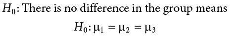
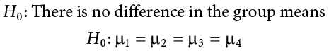
So far we have seen what ANOVA is used for, why we use it, and how we use it. Now we can turn to the formal hypotheses we will be testing. As with before, we have a null and an alternative hypothesis to lay out. Our null hypothesis is still the idea of “no difference” in our data. Because we have multiple group means, we simply list them out as equal to each other:
We list as many  parameters as groups we have. In the example above, we have three groups to test, so we have three parameters in our null hypothesis. If we had more groups, say, four, we would simply add another to the list and give it the appropriate subscript, giving us:
Notice that we do not say that the means are all equal to zero, we only say that they are equal to one another; it does not matter what the actual value is, so long as it holds for all groups equally.
Our alternative hypothesis for ANOVA is a little bit different. Let’s take a look at it and then dive deeper into what it means:

The first difference is obvious: there is no mathematical statement of the alternative hypothesis in ANOVA. This is due to the second difference: we are not saying which group is going to be different, only that at least one will be. Because we do not hypothesize about which mean will be different, there is no way to write it mathematically. Similarly, we do not have directional hypotheses (greater than or less than) like we did in Unit 2. Due to this, our alternative hypothesis is always exactly the same: at least one mean is different.
In Unit 2, we saw that, if we reject the null hypothesis, we can adopt the alternative, and this made it easy to understand what the differences looked like. In ANOVA, we will still adopt the alternative hypothesis as the best explanation of our data if we reject the null hypothesis. However, when we look at the alternative hypothesis, we can see that it does not give us much information. We will know that a difference exists somewhere, but we will not know where that difference is. Is only Group 1 different, but Groups 2 and 3 are the same? Is only Group 2 different? Are all three of them different? Based on just our alternative hypothesis, there is no way to be sure. We will come back to this issue later and see how to find out specific differences. For now, just remember that we are testing for any difference in group means, and it does not matter where that difference occurs.
Now that we have our hypotheses for ANOVA, let’s work through an example. We will continue to use the data from Figure 11.1, Figure 11.2, and Figure 11.3 for continuity.
Example Scores on Job-Application Tests
Our data come from three groups of 10 people each, all of whom applied for a single job opening: those with no college degree, those with a college degree that is not related to the job opening, and those with a college degree from a relevant field. We want to know if we can use this group membership to account for our observed variability and, by doing so, test if there is a difference between our three group means. We will start, as always, with our hypotheses.
Step 1: State the Hypotheses
Our hypotheses are concerned with the means of groups based on education level, so:
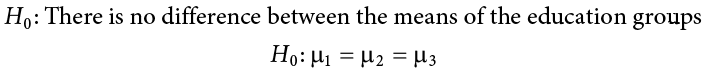
Again, we phrase our null hypothesis in terms of what we are actually testing, and we use a number of population parameters equal to our number of groups. Our alternative hypothesis is always exactly the same.
Step 2: Find the Critical Values
Our test statistic for ANOVA, as we saw above, is F. Because we are using a new test statistic, we will get a new table: the F distribution table, a portion of which is shown in Table 11.2. (The complete F table can be found in Appendix C.)
Table 11.2. Critical values for F (F table).
|
df: Denominator (Within) |
df: Numerator (Between) |
||||||||||||||
|
1 |
2 |
3 |
4 |
5 |
6 |
7 |
8 |
9 |
10 |
11 |
12 |
14 |
16 |
20 |
|
|
1 |
161 |
200 |
216 |
225 |
230 |
234 |
237 |
239 |
241 |
242 |
243 |
244 |
245 |
246 |
248 |
|
2 |
18.51 |
19.00 |
19.16 |
19.25 |
19.30 |
19.33 |
19.36 |
19.37 |
19.38 |
19.39 |
19.40 |
19.41 |
19.42 |
19.43 |
19.44 |
|
3 |
10.13 |
9.55 |
9.28 |
9.12 |
9.01 |
8.94 |
8.88 |
8.84 |
8.81 |
8.78 |
8.76 |
8.74 |
8.71 |
8.69 |
8.66 |
|
4 |
7.71 |
6.94 |
6.59 |
6.39 |
6.26 |
6.16 |
6.09 |
6.04 |
6.00 |
5.96 |
5.93 |
5.91 |
5.87 |
5.84 |
5.80 |
|
5 |
6.61 |
5.79 |
5.41 |
5.19 |
5.05 |
4.95 |
4.88 |
4.82 |
4.78 |
4.74 |
4.70 |
4.68 |
4.64 |
4.60 |
4.56 |
|
6 |
5.99 |
5.14 |
4.76 |
4.53 |
4.39 |
4.28 |
4.21 |
4.15 |
4.10 |
4.06 |
4.03 |
4.00 |
3.96 |
3.92 |
3.87 |
|
7 |
5.59 |
4.74 |
4.35 |
4.12 |
3.97 |
3.87 |
3.79 |
3.73 |
3.68 |
3.63 |
3.60 |
3.57 |
3.52 |
3.49 |
3.44 |
|
8 |
5.32 |
4.46 |
4.07 |
3.84 |
3.69 |
3.58 |
3.50 |
3.44 |
3.39 |
3.34 |
3.31 |
3.28 |
3.23 |
3.20 |
3.15 |
|
9 |
5.12 |
4.26 |
3.86 |
3.63 |
3.48 |
3.37 |
3.29 |
3.23 |
3.18 |
3.13 |
3.10 |
3.07 |
3.02 |
2.98 |
2.93 |
|
10 |
4.96 |
4.10 |
3.71 |
3.48 |
3.33 |
3.22 |
3.14 |
3.07 |
3.02 |
2.97 |
2.94 |
2.91 |
2.86 |
2.82 |
2.77 |
|
11 |
4.84 |
3.98 |
3.59 |
3.36 |
3.20 |
3.09 |
3.01 |
2.95 |
2.90 |
2.86 |
2.82 |
2.79 |
2.74 |
2.70 |
2.65 |
|
12 |
4.75 |
3.88 |
3.49 |
3.26 |
3.11 |
3.00 |
2.92 |
2.85 |
2.80 |
2.76 |
2.72 |
2.69 |
2.64 |
2.60 |
2.54 |
|
13 |
4.67 |
3.80 |
3.41 |
3.18 |
3.02 |
2.92 |
2.84 |
2.77 |
2.72 |
2.67 |
2.63 |
2.60 |
2.55 |
2.51 |
2.46 |
|
14 |
4.60 |
3.74 |
3.34 |
3.11 |
2.96 |
2.85 |
2.77 |
2.70 |
2.65 |
2.60 |
2.56 |
2.53 |
2.48 |
2.44 |
2.39 |
|
15 |
4.54 |
3.68 |
3.29 |
3.06 |
2.90 |
2.79 |
2.70 |
2.64 |
2.59 |
2.55 |
2.51 |
2.48 |
2.43 |
2.39 |
2.33 |
|
16 |
4.49 |
3.63 |
3.24 |
3.01 |
2.85 |
2.74 |
2.66 |
2.59 |
2.54 |
2.49 |
2.45 |
2.42 |
2.37 |
2.33 |
2.28 |
|
17 |
4.45 |
3.59 |
3.20 |
2.96 |
2.81 |
2.70 |
2.62 |
2.55 |
2.50 |
2.45 |
2.41 |
2.38 |
2.33 |
2.29 |
2.23 |
|
18 |
4.41 |
3.55 |
3.16 |
2.93 |
2.77 |
2.66 |
2.58 |
2.51 |
2.46 |
2.41 |
2.37 |
2.34 |
2.29 |
2.25 |
2.19 |
|
19 |
4.38 |
3.52 |
3.13 |
2.90 |
2.74 |
2.63 |
2.55 |
2.48 |
2.43 |
2.38 |
2.34 |
2.31 |
2.26 |
2.21 |
2.15 |
|
20 |
4.35 |
3.49 |
3.10 |
2.87 |
2.71 |
2.60 |
2.52 |
2.45 |
2.40 |
2.35 |
2.31 |
2.28 |
2.23 |
2.18 |
2.12 |
|
21 |
4.32 |
3.47 |
3.07 |
2.84 |
2.68 |
2.57 |
2.49 |
2.42 |
2.37 |
2.32 |
2.28 |
2.25 |
2.20 |
2.15 |
2.09 |
|
22 |
4.30 |
3.44 |
3.05 |
2.82 |
2.66 |
2.55 |
2.47 |
2.40 |
2.35 |
2.30 |
2.26 |
2.23 |
2.18 |
2.13 |
2.07 |
|
23 |
4.28 |
3.42 |
3.03 |
2.80 |
2.64 |
2.53 |
2.45 |
2.38 |
2.32 |
2.28 |
2.24 |
2.20 |
2.14 |
2.10 |
2.04 |
|
24 |
4.26 |
3.40 |
3.01 |
2.78 |
2.62 |
2.51 |
2.43 |
2.36 |
2.30 |
2.26 |
2.22 |
2.18 |
2.13 |
2.09 |
2.02 |
|
25 |
4.24 |
3.38 |
2.99 |
2.76 |
2.60 |
2.49 |
2.41 |
2.34 |
2.28 |
2.24 |
2.20 |
2.15 |
2.11 |
2.06 |
2.00 |
|
26 |
4.22 |
3.37 |
2.98 |
2.74 |
2.59 |
2.47 |
2.39 |
2.32 |
2.27 |
2.22 |
2.18 |
2.15 |
2.10 |
2.05 |
1.99 |
|
27 |
4.21 |
3.35 |
2.96 |
2.73 |
2.57 |
2.46 |
2.37 |
2.30 |
2.25 |
2.20 |
2.16 |
2.13 |
2.08 |
2.03 |
1.97 |
The F table only displays critical values for a = .05. This is because other significance levels are uncommon and so it is not worth it to use up the space to present them. There are now two degrees of freedom we must use to find our critical value: numerator and denominator. These correspond to the numerator and denominator of our test statistic, which, if you look at the ANOVA table presented earlier (Table 11.1), are our Between and Within rows, respectively. The dfB is the “df: Numerator (Between)” because it is the degrees of freedom value used to calculate the Mean Square Between, which in turn is the numerator of our F statistic. Likewise, the dfW is the “df: Denominator (Within)” because it is the degrees of freedom value used to calculate the Mean Square Within, which is our denominator for F.
The formula for dfB is k − 1; remember that k is the number of groups we are assessing. In this example, k = 3 so our dfB = 2. This tells us that we will use the second column, the one labeled 2, to find our critical value. To find the proper row, we simply calculate the dfW, which was N − k. The original prompt told us that we have “three groups of 10 people each,” so our total sample size is 30. This makes our value for dfW = 27. If we follow the second column down to the row for 27, we find that our critical value is 3.35. We use this critical value the same way as we did before: it is our criterion against which we will compare our obtained test statistic to determine statistical significance.
Step 3: Calculate the Test Statistic and Effect Size
Now that we have our hypotheses and the criteria we will use to test them, we can calculate our test statistic. To do this, we will fill in the ANOVA table, working our way from left to right and filling in each cell to get our final answer. We will assume that we are given the SS values as shown below:
|
Source |
SS |
df |
MS |
F |
|
Between |
8246 |
|||
|
Within |
3020 |
|||
|
Total |
These may seem like random numbers, but remember that they are based on the distances between the groups themselves and within each group. Figure 11.4 shows the plot of the data with the group means and grand mean included. If we wanted to, we could use this information, combined with our earlier information that each group has 10 people, to calculate the between-groups sum of squares by hand. However, doing so would take some time, and without the specific values of the data points, we would not be able to calculate our within-groups sum of squares, so we will trust that these values are the correct ones.
Figure 11.4. Means. (“Job Test Scores Group Means” by Judy Schmitt is licensed under CC BY-NC-SA 4.0.)
We were given the sums of squares values for our first two rows, so we can use those to calculate the total sum of squares.
|
Source |
SS |
df |
MS |
F |
|
Between |
8246 |
|||
|
Within |
3020 |
|||
|
Total |
11266 |
We also calculated our degrees of freedom earlier, so we can fill in those values. Additionally, we know that the total degrees of freedom is N − 1, which is 29. This value of 29 is also the sum of the other two degrees of freedom, so everything checks out.
|
Source |
SS |
df |
MS |
F |
|
Between |
8246 |
2 |
||
|
Within |
3020 |
27 |
||
|
Total |
11266 |
29 |
Now we have everything we need to calculate our mean squares. Our MS values for each row are just the SS divided by the df for that row, giving us:
|
Source |
SS |
df |
MS |
F |
|
Between |
8246 |
2 |
4123 |
|
|
Within |
3020 |
27 |
111.85 |
|
|
Total |
11266 |
29 |
Remember that we do not calculate a Total Mean Square, so we leave that cell blank. Finally, we have the information we need to calculate our test statistic. F is our MSB divided by MSW.
|
Source |
SS |
df |
MS |
F |
|
Between |
8246 |
2 |
4123 |
36.86 |
|
Within |
3020 |
27 |
111.85 |
|
|
Total |
11266 |
29 |
So, working our way through the table, given only two SS values and the sample size and group size from before, we calculate our test statistic to be Fobt = 36.86, which we will compare to the critical value in Step 4.
Effect Size: Variance Explained
Recall that the purpose of ANOVA is to take observed variability and see if we can explain those differences based on group membership. To that end, our effect size will be just that: the variance explained. You can think of variance explained as the proportion or percent of the differences we are able to account for based on our groups. We know that the overall observed differences are quantified as the total sum of squares, and that our observed effect of group membership is the between-groups sum of squares. Our effect size, therefore, is the ratio of these two sums of squares. Specifically:
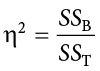
The effect size h2 is called “eta-squared” and represents variance explained. For our example, our values give an effect size of:
So, we are able to explain 73% of the variance in job-test scores based on education. This is, in fact, a huge effect size, and most of the time we will not explain nearly that much variance. Our guidelines for the size of our effects are:
|
|
Size |
|
.01 |
Small |
|
.09 |
Medium |
|
.25 |
Large |
 2
2So, we found that not only do we have a statistically significant result, but that our observed effect was very large! However, we still do not know specifically which groups are different from each other. It could be that they are all different, or that only those job seekers who have a relevant degree are different from the others, or that only those who have no degree are different from the others. To find out which is true, we need to do a special analysis called a post hoc test.
Step 4: Make the Decision
Our obtained test statistic was calculated to be Fobt = 36.86 and our critical value was found to be F* = 3.35. Our obtained statistic is larger than our critical value, so we can reject the null hypothesis.
Reject H0. The results of the ANOVA indicated that there were significant differences in job skills test scores for applicants in each of the three education groups, and the effect size was large, F(2, 27) = 36.86, p < .05, h2 = .73. Post hoc tests (see the next section) were performed to determine where the differences were.
Notice that when we report F, we include both degrees of freedom. We always report the numerator and then the denominator, separated by a comma. We must also note that, because we were only testing for any difference, we cannot yet conclude which groups are different from the others. To do so, we need to perform a post hoc test.
Post Hoc Tests
A post hoc test is used only after we find a statistically significant result and need to determine where our differences truly came from. The term post hoc comes from the Latin for “after the event.” Many different post hoc tests have been developed, and most of them will give us similar answers. We will only focus here on the most commonly used ones. We will also only discuss the concepts behind each and will not worry about calculations.
Bonferroni Test
A Bonferroni test is perhaps the simplest post hoc analysis. A Bonferroni test is a series of t tests performed on each pair of groups. As we discussed earlier, the number of groups quickly increases the number of comparisons, which inflates Type I error rates. To avoid this, a Bonferroni test divides our significance level by the number of comparisons we are making so that when they are all run, they sum back up to our original Type I error rate. Once we have our new significance level, we simply run independent samples t tests to look for differences between our pairs of groups. This adjustment is sometimes called a Bonferroni Correction, and it is easy to do by hand if we want to compare obtained p values to our new corrected level, but it is more difficult to do when using critical values like we do for our analyses, so we will leave our discussion of it to that.
Tukey’s Honestly Significant Difference
Tukey’s honestly significant difference (HSD) is a popular post hoc analysis that, like Bonferroni’s, makes adjustments based on the number of comparisons; however, it makes adjustments to the test statistic when running the comparisons of two groups. These comparisons give us an estimate of the difference between the groups and a confidence interval for the estimate. We use this confidence interval in the same way we use a confidence interval for a regular independent samples t test: if it contains 0.00, the groups are not different, but if it does not contain 0.00 then the groups are different.
Below are the differences between the group means and the Tukey’s HSD confidence intervals for the differences:
|
Comparison |
Difference |
Tukey’s HSD CI |
|
None vs. relevant |
40.60 |
(28.87, 52.33) |
|
None vs. unrelated |
19.50 |
(7.77, 31.23) |
|
Relevant vs. unrelated |
21.10 |
(9.37, 32.83) |
As we can see, none of these intervals contain 0.00, so we can conclude that all three groups are different from one another.
Scheffé Test
Another common post hoc test is the Scheffé test. Like Tukey’s HSD, the Scheffé test adjusts the test statistic for how many comparisons are made, but it does so in a slightly different way. The result is a test that is “conservative,” which means that it is less likely to commit a Type I error, but this comes at the cost of less power to detect effects. We can see this by looking at the confidence intervals that the Scheffé test gives us:
|
Comparison |
Difference |
Scheffé CI |
|
None vs. relevant |
40.60 |
(28.35, 52.85) |
|
None vs. unrelated |
19.50 |
(7.25, 31.75) |
|
Relevant vs. unrelated |
21.10 |
(8.85, 33.35) |
As we can see, these are slightly wider than the intervals we got from Tukey’s HSD. This means that, all other things being equal, they are more likely to contain zero. In our case, however, the results are the same, and we again conclude that all three groups differ from one another.
There are many more post hoc tests than just these three, and they all approach the task in different ways, with some being more conservative and others being more powerful. In general, though, they will give highly similar answers. What is important here is to be able to interpret a post hoc analysis. If you are given post hoc analysis confidence intervals, like the ones seen above, read them the same way we read confidence intervals in Chapter 10. If they contain zero, there is no difference; if they do not contain zero, there is a difference.
Other ANOVA Designs
We have only just scratched the surface on ANOVA in this chapter. There are many other variations available for the one-way ANOVA presented here. There are also other types of ANOVAs that you are likely to encounter. The first is called a factorial ANOVA. A factorial ANOVA uses multiple grouping variables, not just one, to look for group mean differences. Just as there is no limit to the number of groups in a one-way ANOVA, there is no limit to the number of grouping variables in a factorial ANOVA, but it becomes very difficult to find and interpret significant results with many factors, so usually they are limited to two or three grouping variables with only a small number of groups in each.
Another ANOVA is called a repeated measures ANOVA. This is an extension of a related samples t test, but in this case we are measuring each person three or more times to look for a change. We can even combine both of these advanced ANOVAs into mixed designs to test very specific and valuable questions. These topics are far beyond the scope of this text, but you should know about their existence. Our treatment of ANOVA here is a small first step into a much larger world!
Exercises
- What sources of variability are analyzed in an ANOVA?
- What does rejecting the null hypothesis in ANOVA tell us? What does it not tell us?
- What is the purpose of post hoc tests?
- Based on the ANOVA table below, do you reject or fail to reject the null hypothesis? What is the effect size?
Source
SS
df
MS
F
Between
60.72
3
20.24
3.88
Within
213.61
41
5.21
Total
274.33
44
- Finish filling out the following ANOVA tables:
- k = 4
Source
SS
df
MS
F
Between
87.40
Within
Total
199.22
33
- N = 14
Source
SS
df
MS
F
Between
2
14.10
Within
Total
64.65
-
Source
SS
df
MS
F
Between
2
42.36
Within
54
2.48
Total
- k = 4
- You know that stores tend to charge different prices for similar or identical products, and you want to test whether or not these differences are, on average, statistically significantly different. You go online and collect data from three different stores, gathering information on 15 products at each store. You find that the average prices at each store are: Store 1 M = $27.82, Store 2 M = $38.96, and Store 3 M = $24.53. Based on the overall variability in the products and the variability within each store, you find the following values for the sums of squares: SST = 683.22, SSW = 441.19. Complete the ANOVA table and use the four-step hypothesis testing procedure to see if there are systematic price differences between the stores.
- You and your friend are debating which type of candy is the best. You find data on the average rating for hard candy (e.g., Jolly Ranchers, M = 3.60), chewable candy (e.g., Starburst, M = 4.20), and chocolate (e.g., Snickers, M = 4.40); each type of candy was rated by 30 people. Test for differences in average candy rating using SSB = 16.18 and SSW = 28.74.
- Administrators at a university want to know if students in different majors are more or less extroverted than others. They provide you with data they have for English majors (M = 3.78, n = 45), History majors (M = 2.23, n = 40), Psychology majors (M = 4.41, n = 51), and Math majors (M = 1.15, n = 28). You find the SSB = 75.80 and SSW = 47.40 and test at a = .05.
- You are assigned to run a study comparing a new medication (M = 17.47, n = 19), an existing medication (M = 17.94, n = 18), and a placebo (M = 13.70, n = 20), with higher scores reflecting better outcomes. Use SSB = 210.10 and SSW = 133.90 to test for differences.
- Attributions (explanations) for human behavior are known to vary across cultures. Researchers investigated whether South Korean, Korean immigrant, and Korean American school children’s attributions for their academic outcomes differed. Each student was presented with 5 negative academic outcomes (such as failing a test) and asked to choose whether they believed the outcome was due to lack of effort or lack of ability. Data are the number of outcomes for which students chose “lack of effort.” Test the hypothesis at the a = .05 level using the four-step hypothesis testing procedure.
South Korean
Korean Immigrant
Korean American
5
4
3
4
3
2
3
4
1
2
4
1
5
3
5
4
2
4
5
5
3
4
1
3
Answers to Odd-Numbered Exercises
1)
Between-groups and within-groups variability are analyzed in an ANOVA.
3)
Post hoc tests are run if we reject the null hypothesis in ANOVA; they tell us which specific group differences are significant.
5)
Finish filling out the following ANOVA tables:
a)
k = 4
|
Source |
SS |
df |
MS |
F |
|
Between |
87.40 |
3 |
29.13 |
7.81 |
|
Within |
111.82 |
30 |
3.73 |
|
|
Total |
199.22 |
33 |
b)
N = 14
|
Source |
SS |
df |
MS |
F |
|
Between |
28.20 |
2 |
14.10 |
4.26 |
|
Within |
36.45 |
11 |
3.31 |
|
|
Total |
64.65 |
13 |
c)
|
Source |
SS |
df |
MS |
F |
|
Between |
210.10 |
2 |
105.05 |
42.36 |
|
Within |
133.92 |
54 |
2.48 |
|
|
Total |
344.02 |
7)
Step 1: H₀: ₁ = ₂ = ₃ “There is no difference in average rating of candy quality,” HA: “At least one mean is different.”
Step 2: 3 groups and 90 total observations yields dfnum = 2 and dfden = 87, a = .05, F* = 3.11
Step 3: Based on the given SSB and SSW and the computed df from Step 2:
|
Source |
SS |
df |
MS |
F |
|
Between |
16.18 |
2 |
8.09 |
24.52 |
|
Within |
28.74 |
87 |
0.33 |
|
|
Total |
44.92 |
89 |
h2 = 16.18/44.92 = .36
Step 4: F > F*, Reject H0. Based on the data in our 3 groups, we can say that there is a statistically significant difference in the quality of different types of candy, and the effect size is large, F(2,87) = 24.52, p < .05, h2 = .36.
