8 Chapter 8: Introduction to t Tests

In Chapter 7, we made a big leap from basic descriptive statistics into full hypothesis testing and inferential statistics. For the rest of the unit, we will be learning new tests, each of which is just a small adjustment on the test before it. In this chapter, we will learn about the first of three t tests, and we will learn a new method of testing the null hypothesis: confidence intervals.

The t Statistic

In Chapter 7, we were introduced to hypothesis testing using the z statistic for sample means that we learned in Unit 1. This was a useful way to link the material and ease us into the new way to looking at data, but it isn’t a very common test because it relies on knowing the population’s standard deviation, s, which is rarely going to be the case. Instead, we will estimate that parameter s using the sample statistic s in the same way that we estimate using ( will still appear in our formulas because we suspect something about its value and that is what we are testing). Our new statistic is called t, and for testing one population mean using a single sample (called a one-sample t test) it takes the form:

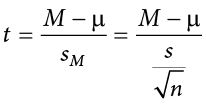
Notice that t looks almost identical to z; this is because they test the exact same thing: the value of a sample mean compared to what we expect of the population. The only difference is that the standard error is now denoted to indicate that we use the sample statistic for standard deviation, s, instead of the population parameter s. The process of using and interpreting the standard error and the full test statistic remain exactly the same.

In Chapter 3 we learned that the formulas for sample standard deviation and population standard deviation differ by one key factor: the denominator for the parameter is but the denominator for the statistic is N − 1, also known as degrees of freedom, df. Because we are using a new measure of spread, we can no longer use the standard normal distribution and the z table to find our critical values. For t tests, we will use the t distribution and t table to find these values.

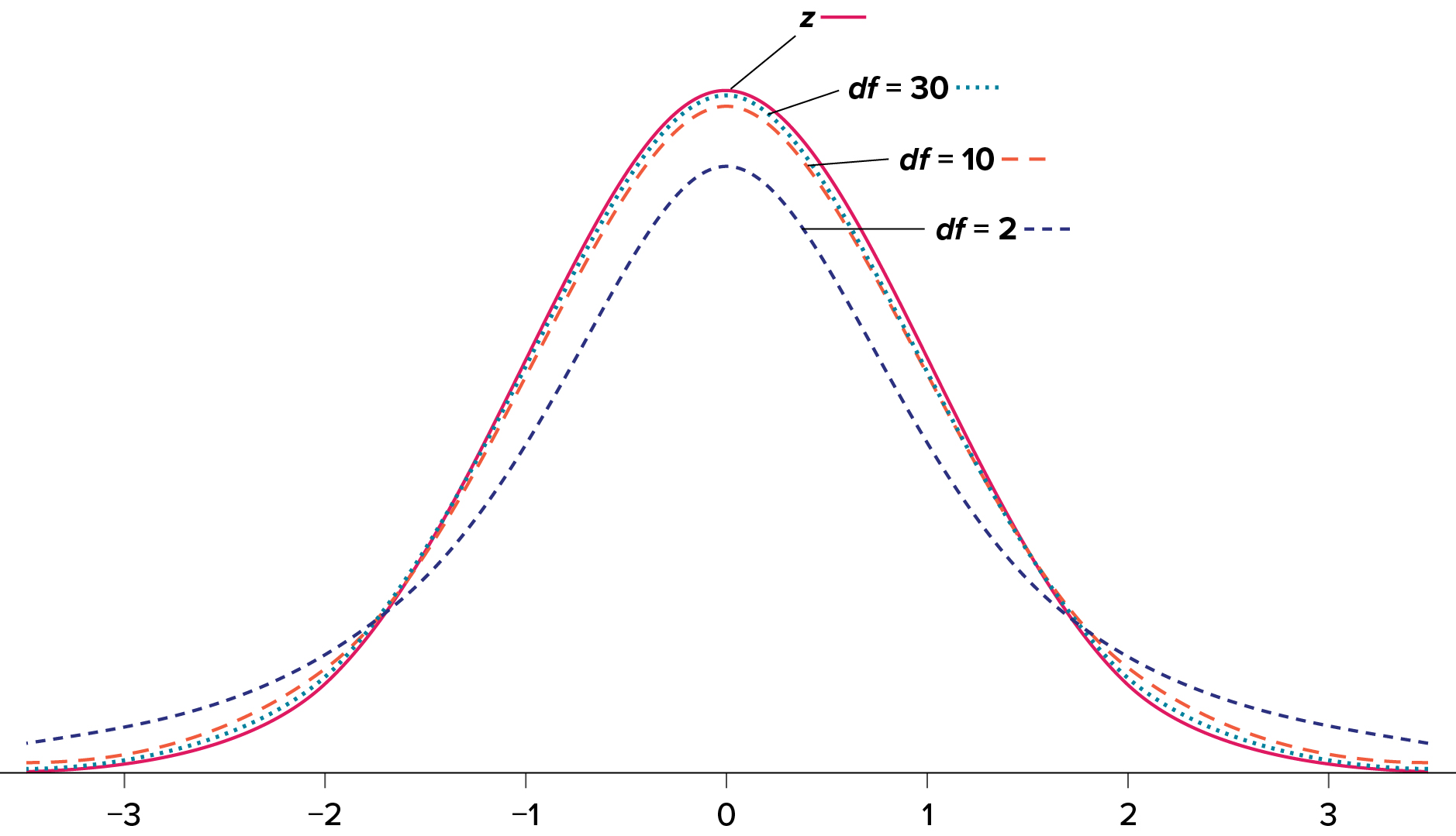
The t distribution, like the standard normal distribution, is symmetric and normally distributed with a mean of 0 and standard error (as the measure of standard deviation for sampling distributions) of 1. However, because the calculation of standard error uses degrees of freedom, there will be a different t distribution for every degree of freedom. Luckily, they all work exactly the same, so in practice this difference is minor.

Figure 8.1 shows four curves: a normal distribution curve labeled z, and three t distribution curves for 2, 10, and 30 degrees of freedom. Two things should stand out: First, for lower degrees of freedom (e.g., 2), the tails of the distribution are much fatter, meaning the a larger proportion of the area under the curve falls in the tail. This means that we will have to go farther out into the tail to cut off the portion corresponding to 5% or a = .05, which will in turn lead to higher critical values. Second, as the degrees of freedom increase, we get closer and closer to the z curve. Even the distribution with df = 30, corresponding to a sample size of just 31 people, is nearly indistinguishable from z. In fact, a t distribution with infinite degrees of freedom (theoretically, of course) is exactly the standard normal distribution. Because of this, the bottom row of the t table also includes the critical values for z tests at the specific significance levels. Even though these curves are very close, it is still important to use the correct table and critical values, because small differences can add up quickly.

The t distribution table lists critical values for one- and two-tailed tests at several levels of significance, arranged into columns. The rows of the t table list degrees of freedom up to df = 100 in order to use the appropriate distribution curve. It does not, however, list all possible degrees of freedom in this range, because that would take too many rows. Above df = 40, the rows jump in increments of 10. If a problem requires you to find critical values and the exact degrees of freedom is not listed, you always round down to the next smallest number. For example, if you have 48 people in your sample, the degrees of freedom are N − 1 = 48 − 1 = 47; however, 47 doesn’t appear on our table, so we round down and use the critical values for df = 40, even though 50 is closer. We do this because it avoids inflating Type I error (false positives, see Chapter 7) by using criteria that are too lax.

Hypothesis Testing with t

Hypothesis testing with the t statistic works exactly the same way as z tests did, following the four-step process of (1) stating the hypotheses, (2) finding the critical values, (3) computing the test statistic and effect size, and (4) making the decision.

Example Oil Change Speed

We will work though an example: Let’s say that you move to a new city and find an auto shop to change your oil. Your old mechanic did the job in about 30 minutes (although you never paid close enough attention to know how much that varied), and you suspect that your new shop takes much longer. After four oil changes, you think you have enough evidence to demonstrate this.

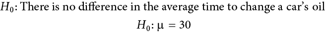
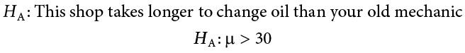
Step 1: State the Hypotheses

Our hypotheses for one-sample t tests are identical to those we used for z tests. We still state the null and alternative hypotheses mathematically in terms of the population parameter and written out in readable English. For our example:

Step 2: Find the Critical Values

As noted above, our critical values still delineate the area in the tails under the curve corresponding to our chosen level of significance. Because we have no reason to change significance levels, we will use a = .05, and because we suspect a direction of effect, we have a one-tailed test. To find our critical values for t, we need to add one more piece of information: the degrees of freedom. For this example:

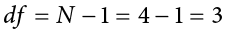
Going to our t table, a portion of which is found in Table 8.1, we locate the column corresponding to our one-tailed significance level of .05 and find where it intersects with the row for 3 degrees of freedom. As we can see in Table 8.1, our critical value is t* = 2.353. (The complete t table can be found in Appendix B.)

Table 8.1. t distribution table (t table).

df	Proportion (a) in One tail
	.25	.20	.15	.10	.05	.025	.01	.005	.0005
	Proportion (a) in Two tails combined
	.50	.40	.30	.20	.10	.05	.02	.01	.001
1	1.000	1.376	1.963	3.078	6.314	12.706	31.821	63.657	636.578
2	0.816	1.061	1.386	1.886	2.920	4.303	6.965	9.925	31.600
3	0.765	1.978	1.250	1.638	2.353	3.182	4.541	5.841	12.924
4	0.741	1.941	1.190	1.533	2.132	2.776	3.747	4.604	8.610
5	0.727	0.920	1.156	1.476	2.015	2.571	3.365	4.032	6.869

Adapted from “Tabla t” by Jsmura/Wikimedia Commons, CC BY-SA 4.0.

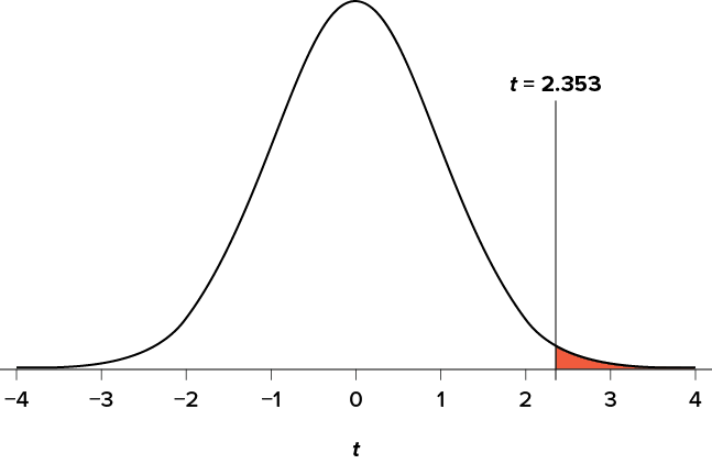
We can then shade this region on our t distribution to visualize our rejection region (Figure 8.2).

Step 3: Calculate the Test Statistic and Effect Size

The four wait times you experienced for your oil changes at the new shop were 46 minutes, 58 minutes, 40 minutes, and 71 minutes. We will use these to calculate and s by first filling in the sum of squares in Table 8.2.

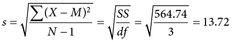
After filling in the first row to get ΣX = 215, we find that the mean is M = 53.75 (215 divided by sample size 4), which allows us to fill in the rest of the table to get our sum of squares SS = 564.74, which we then plug in to the formula for standard deviation from Chapter 3:

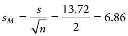
Next, we take this value and plug it in to the formula for standard error:

And, finally, we put the standard error, sample mean, and null hypothesis value into the formula for our test statistic t:

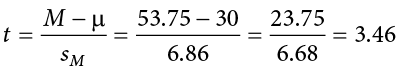
This may seem like a lot of steps, but it is really just taking our raw data to calculate one value at a time and carrying that value forward into the next equation: data → sample size/degrees of freedom → mean → sum of squares → standard deviation → standard error → test statistic. At each step, we simply match the symbols of what we just calculated to where they appear in the next formula to make sure we are plugging everything in correctly.

Next we need to calculate an effect size, which is still Cohen’s d, but now we use s in place of s:

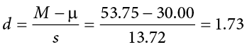
This is a large effect. It should also be noted that for some things, like the minutes in our current example, we can also interpret the magnitude of the difference we observed (23 minutes and 45 seconds) as an indicator of importance since time is a familiar metric.

Step 4: Make the Decision

Now that we have our critical value and test statistic, we can make our decision using the same criteria we used for a z test. Our obtained t statistic was t = 3.46 and our critical value was t* = 2.353: t > t*, so we reject the null hypothesis and conclude:

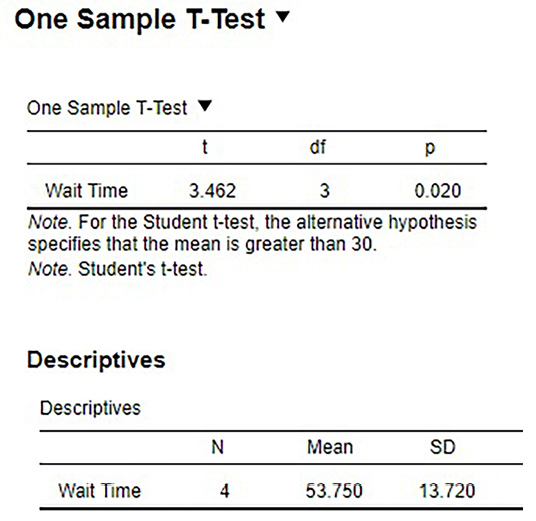
Based on our four oil changes, the new mechanic takes longer on average (M = 53.75, SD = 13.72) to change oil than our old mechanic, and the effect size was large, t(3) = 3.46, p < .05, d = 1.74.

Notice that we also include the degrees of freedom in parentheses next to t. Figure 8.3 shows the output from JASP.

Confidence Intervals

Up to this point, we have learned how to estimate the population parameter for the mean using sample data and a sample statistic. From one point of view, this makes sense: we have one value for our parameter so we use a single value (called a point estimate) to estimate it. However, we have seen that all statistics have sampling error and that the value we find for the sample mean will bounce around based on the people in our sample, simply due to random chance. Thinking about estimation from this perspective, it would make more sense to take that error into account rather than relying just on our point estimate. To do this, we calculate what is known as a confidence interval.

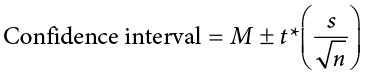
A confidence interval starts with our point estimate and then creates a range of scores considered plausible based on our standard deviation, our sample size, and the level of confidence with which we would like to estimate the parameter. This range, which extends equally in both directions away from the point estimate, is called the margin of error. We calculate the margin of error by multiplying our two-tailed critical value by our standard error:

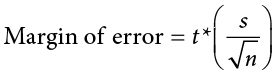
One important consideration when calculating the margin of error is that it can only be calculated using the critical value for a two-tailed test. This is because the margin of error moves away from the point estimate in both directions, so a one-tailed value does not make sense.

The critical value we use will be based on a chosen level of confidence, which is equal to 1 − a. Thus, a 95% level of confidence corresponds to a = .05. Thus, at the .05 level of significance, we create a 95% confidence interval. How to interpret that is discussed further on.

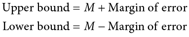
Once we have our margin of error calculated, we add it to our point estimate for the mean to get an upper bound to the confidence interval and subtract it from the point estimate for the mean to get a lower bound for the confidence interval:

or simply:

To write out a confidence interval, we always use round brackets (i.e., parentheses) and put the lower bound, a comma, and the upper bound:

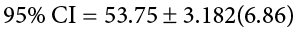
Let’s see what this looks like with some actual numbers by taking our oil change data and using it to create a 95% confidence interval estimating the average length of time it takes at the new mechanic. We already found that our average was M = 53.75 and our standard error was = 6.86. We also found a critical value to test our hypothesis, but remember that we were testing a one-tailed hypothesis, so that critical value won’t work. To see why that is, look at the column headers on the t table. The column for one-tailed a = .05 is the same as a two-tailed a = .10. If we used the old critical value, we’d actually be creating a 90% confidence interval (1.00 − 0.10 = 0.90, or 90%). To find the correct value, we use the column for two-tailed a = .05 and, again, the row for 3 degrees of freedom, to find t* = 3.182.

Now we have all the pieces we need to construct our confidence interval:

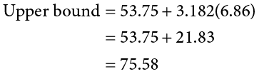
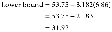
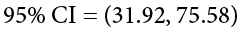
So we find that our 95% confidence interval runs from 31.92 minutes to 75.58 minutes, but what does that actually mean? The range (31.92, 75.58) represents values of the mean that we consider reasonable or plausible based on our observed data. It includes our point estimate of the mean, M = 53.75, in the center, but it also has a range of values that could also have been the case based on what we know about how much these scores vary (i.e., our standard error).

It is very tempting to also interpret this interval by saying that we are 95% confident that the true population mean falls within the range (31.92, 75.58), but this is not true. The reason it is not true is that phrasing our interpretation this way suggests that we have firmly established an interval and the population mean does or does not fall into it, suggesting that our interval is firm and the population mean will move around. However, the population mean is an absolute that does not change; it is our interval that will vary from data collection to data collection, even taking into account our standard error. The correct interpretation, then, is that we are 95% confident that the range (31.92, 75.58) brackets the true population mean. This is a very subtle difference, but it is an important one.

Hypothesis Testing with Confidence Intervals

As a function of how they are constructed, we can also use confidence intervals to test hypotheses. However, we are limited to testing two-tailed hypotheses only, because of how the intervals work, as discussed above.

Once a confidence interval has been constructed, using it to test a hypothesis is simple. If the range of the confidence interval brackets (or contains, or is around) the null hypothesis value, we fail to reject the null hypothesis. If it does not bracket the null hypothesis value (i.e., if the entire range is above the null hypothesis value or below it), we reject the null hypothesis. The reason for this is clear if we think about what a confidence interval represents. Remember: a confidence interval is a range of values that we consider reasonable or plausible based on our data. Thus, if the null hypothesis value is in that range, then it is a value that is plausible based on our observations. If the null hypothesis is plausible, then we have no reason to reject it. Thus, if our confidence interval brackets the null hypothesis value, thereby making it a reasonable or plausible value based on our observed data, then we have no evidence against the null hypothesis and fail to reject it. However, if we build a confidence interval of reasonable values based on our observations and it does not contain the null hypothesis value, then we have no empirical (observed) reason to believe the null hypothesis value and therefore reject the null hypothesis.

Example Friendliness

You hear that the national average on a measure of friendliness is 38 points. You want to know if people in your community are more or less friendly than people nationwide, so you collect data from 30 random people in town to look for a difference. We’ll follow the same four-step hypothesis-testing procedure as before.

Step 1: State the Hypotheses

We will start by laying out our null and alternative hypotheses:

Step 2: Find the Critical Values

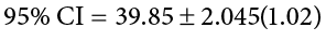
We need our critical values in order to determine the width of our margin of error. We will assume a significance level of a = .05 (which will give us a 95% CI). From the t table, a two-tailed critical value at a = .05 with 29 degrees of freedom (N − 1 = 30 − 1 = 29) is t* = 2.045.

Step 3: Calculate the Confidence Interval

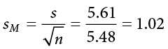
Now we can construct our confidence interval. After we collect our data, we find that the average person in our community scored 39.85, or M = 39.85, and our standard deviation was s = 5.61. First, we need to use this standard deviation, plus our sample size of N = 30, to calculate our standard error:

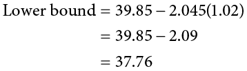
Now we can put that value, our point estimate for the sample mean, and our critical value from Step 2 into the formula for a confidence interval:

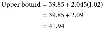
Step 4: Make the Decision

Finally, we can compare our confidence interval to our null hypothesis value. The null value of 38 is higher than our lower bound of 37.76 and lower than our upper bound of 41.94. Thus, the confidence interval brackets our null hypothesis value, and we fail to reject the null hypothesis:

Fail to reject H0. Based on our sample of 30 people, our community is not different in average friendliness (M = 39.85, SD = 5.61) than the nation as a whole, 95% CI = (37.76, 41.94).

Note that we don’t report a test statistic or p value because that is not how we tested the hypothesis, but we do report the value we found for our confidence interval.

An important characteristic of hypothesis testing is that both methods will always give you the same result. That is because both are based on the standard error and critical values in their calculations. To check this, we can calculate a t statistic for the example above and find it to be t = 1.81, which is smaller than our critical value of 2.045 and fails to reject the null hypothesis.

Confidence Intervals Using z

Confidence intervals can also be constructed using z score criteria, if one knows the population standard deviation. The format, calculations, and interpretation are all exactly the same, only replacing t* with z* and with .

Exercises

1. What is the difference between a z test and a one-sample t test?
2. What does a confidence interval represent?
3. What is the relationship between a chosen level of confidence for a confidence interval and how wide that interval is? For instance, if you move from a 95% CI to a 90% CI, what happens? Hint: look at the t table to see how critical values change when you change levels of significance.
4. Construct a confidence interval around the sample mean M = 25 for the following conditions:
   1. N = 25, s = 15, 95% confidence level
   2. N = 25, s = 15, 90% confidence level
   3. = 4.5, a = .05, df = 20
   4. s = 12, df = 16 (yes, that is all the information you need)
5. True or false: A confidence interval represents the most likely location of the true population mean.
6. You hear that college campuses may differ from the general population in terms of political affiliation, and you want to use hypothesis testing to see if this is true and, if so, how big the difference is. You know that the average political affiliation in the nation is = 4.00 on a scale of 1.00 to 7.00, so you gather data from 150 college students across the nation to see if there is a difference. You find that the average score is 3.76 with a standard deviation of 1.52. Use a one-sample t test to see if there is a difference at the a = .05 level.
7. You hear a lot of talk about increasing global temperature, so you decide to see for yourself if there has been an actual change in recent years. You know that the average land temperature from 1951-1980 was 8.79 degrees Celsius. You find annual average temperature data from 1981–2017 and decide to construct a 99% confidence interval (because you want to be as sure as possible and look for differences in both directions, not just one) using this data to test for a difference from the previous average.
   

   Year	Temp
   1981	9.301
   1982	8.788
   1983	9.173
   1984	8.824
   1985	8.799
   1986	8.985
   1987	9.141
   1988	9.345
   1989	9.076
   1990	9.378
   1991	9.336
   1992	8.974
   1993	9.008
   1994	9.175
   1995	9.484
   1996	9.168
   1997	9.326
   1998	9.660
   1999	9.406
   2000	9.332
   2001	9.542
   2002	9.695
   2003	9.649
   2004	9.451
   2005	9.829
   2006	9.662
   2007	9.876
   2008	9.581
   2009	9.657
   2010	9.828
   2011	9.650
   2012	9.635
   2013	9.753
   2014	9.714
   2015	9.962
   2016	10.160
   2017	10.049

8. Determine whether you would reject or fail to reject the null hypothesis in the following situations:
   1. t = 2.58, N = 21, two-tailed test at a = .05
   2. t = 1.99, N = 49, one-tailed test at a = .01
   3. = 47.82, 99% CI = (48.71, 49.28)
   4. = 0, 95% CI = (−0.15, 0.20)
9. You are curious about how people feel about craft beer, so you gather data from 55 people in the city on whether or not they like it. You code your data so that 0 is neutral, positive scores indicate liking craft beer, and negative scores indicate disliking craft beer. You find that the average opinion was M = 1.10 and the spread was s = 0.40, and you test for a difference from 0 at the a = .05 level.
10. You want to know if college students have more stress in their daily lives than the general population ( = 12), so you gather data from 25 people to test your hypothesis. Your sample has an average stress score of M = 13.11 and a standard deviation of s = 3.89. Use a one-sample t test to see if there is a difference.

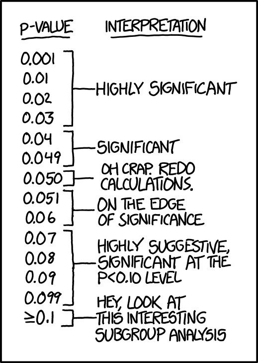
“P-Values” by Randall Munroe/xkcd.com is licensed under CC BY-NC 2.5.)