4 Chapter 4: z Scores and the Standard Normal Distribution

We now understand how to describe and present our data visually and numerically. These simple tools, and the principles behind them, will help you interpret information presented to you and understand the basics of a variable. Moving forward, we now turn our attention to how scores within a distribution are related to one another, how to precisely describe a score’s location within the distribution, and how to compare scores from different distributions.

Normal Distributions

The normal distribution is the most important and most widely used distribution in statistics. It is sometimes called the “bell curve,” although the tonal qualities of such a bell would be less than pleasing. It is also called the “Gaussian curve” of Gaussian distribution after the mathematician Karl Friedrich Gauss.

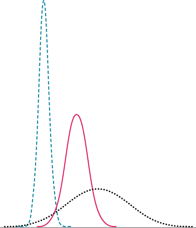
Strictly speaking, it is not correct to talk about “the normal distribution” since there are many normal distributions. Normal distributions can differ in their means and in their standard deviations. Figure 4.1 shows three normal distributions. The blue (left-most) distribution has a mean of −3 and a standard deviation of 0.5, the distribution in red (the middle distribution) has a mean of 0 and a standard deviation of 1, and the black (right-most) distribution has a mean of 2 and a standard deviation of 3. These as well as all other normal distributions are symmetric with relatively more values at the center of the distribution and relatively few in the tails. What is consistent about all normal distribution is the shape and the proportion of scores within a given distance along the x-axis. We will focus on the standard normal distribution (also known as the unit normal distribution), which has a mean of 0 and a standard deviation of 1 (i.e., the red distribution in Figure 4.1).

Seven features of normal distributions are listed below.

1. Normal distributions are symmetric around their mean.
2. The mean, median, and mode of a normal distribution are equal.
3. The area under the normal curve is equal to 1.0.
4. Normal distributions are denser in the center and less dense in the tails.
5. Normal distributions are defined by two parameters, the mean () and the standard deviation (s).
6. 68% of the area of a normal distribution is within one standard deviation of the mean.
7. Approximately 95% of the area of a normal distribution is within two standard deviations of the mean.

These properties enable us to use the normal distribution to understand how scores relate to one another within and across a distribution. But first, we need to learn how to calculate the standardized score that makes up a standard normal distribution.

Z Scores

A z score is a standardized version of a raw score (x) that gives information about the relative location of that score within its distribution. The formula for converting a raw score into a z score is

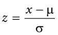
for values from a population and

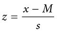
for values from a sample.

As you can see, z scores combine information about where the distribution is located (the mean/center) with how wide the distribution is (the standard deviation/spread) to interpret a raw score (x). Specifically, z scores will tell us how far the score is away from the mean in units of standard deviations and in what direction.

The value of a z score has two parts: the sign (positive or negative) and the magnitude (the actual number). The sign of the z score tells you in which half of the distribution the z score falls: a positive sign (or no sign) indicates that the score is above the mean and on the right-hand side or upper end of the distribution, and a negative sign tells you the score is below the mean and on the left-hand side or lower end of the distribution. The magnitude of the number tells you, in units of standard deviations, how far away the score is from the center or mean. The magnitude can take on any value between negative and positive infinity, but for reasons we will see soon, they generally fall between −3 and 3.

Let’s look at some examples. A z score value of −1.0 tells us that this z score is 1 standard deviation (because of the magnitude 1.0) below (because of the negative sign) the mean. Similarly, a z score value of 1.0 tells us that this z score is 1 standard deviation above the mean. Thus, these two scores are the same distance away from the mean but in opposite directions. A z score of −2.5 is two-and-a-half standard deviations below the mean and is therefore farther from the center than both of the previous scores, and a z score of 0.25 is closer than all of the ones before. In Unit 2, we will learn to formalize the distinction between what we consider “close to” the center or “far from” the center. For now, we will use a rough cut-off of 1.5 standard deviations in either direction as the difference between close scores (those within 1.5 standard deviations or between z = −1.5 and z = 1.5) and extreme scores (those farther than 1.5 standard deviations—below z = −1.5 or above z = 1.5).

We can also convert raw scores into z scores to get a better idea of where in the distribution those scores fall. Let’s say we get a score of 68 on an exam. We may be disappointed to have scored so low, but perhaps it was just a very hard exam. Having information about the distribution of all scores in the class would be helpful to put some perspective on ours. We find out that the class got an average score of 54 with a standard deviation of 8. To find out our relative location within this distribution, we simply convert our test score into a z score.

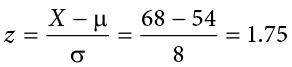
We find that we are 1.75 standard deviations above the average, above our rough cut-off for close and far. Suddenly our 68 is looking pretty good!

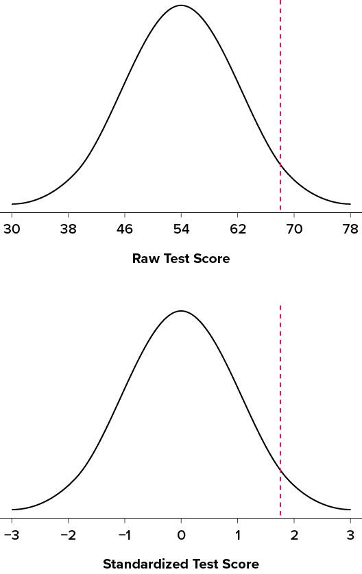
Figure 4.2 shows both the raw score and the z score on their respective distributions. Notice that the red line indicating where each score lies is in the same relative spot for both. This is because transforming a raw score into a z score does not change its relative location, it only makes it easier to know precisely where it is.

z Scores are also useful for comparing scores from different distributions. Let’s say we take the SAT and score 501 on both the math and critical reading sections. Does that mean we did equally well on both? Scores on the math portion are distributed normally with a mean of 511 and standard deviation of 120, so our z score on the math section is

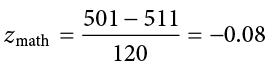
which is just slightly below average (note the use of “math” as a subscript; subscripts are used when presenting multiple versions of the same statistic in order to know which one is which and have no bearing on the actual calculation). The critical reading section has a mean of 495 and standard deviation of 116, so

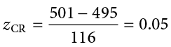
So even though we were almost exactly average on both tests, we did a little bit better on the critical reading portion relative to other people.

Finally, z scores are incredibly useful if we need to combine information from different measures that are on different scales. Let’s say we give a set of employees a series of tests on things like job knowledge, personality, and leadership. We may want to combine these into a single score we can use to rate employees for development or promotion, but look what happens when we take the average of raw scores from different scales, as shown in Table 4.1.

Because the job knowledge scores were so big and the scores were so similar, they overpowered the other scores and removed almost all variability in the average. However, if we standardize these scores into z scores, our averages retain more variability and it is easier to assess differences between employees, as shown in Table 4.2.

Setting the Scale of a Distribution

Another convenient characteristic of z scores is that they can be converted into any “scale” that we would like. Here, the term scale means how far apart the scores are (their spread) and where they are located (their central tendency). This can be very useful if we don’t want to work with negative numbers or if we have a specific range we would like to present. The formulas for transforming z to x are:

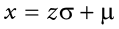
for a population and

for a sample. Notice that these are just simple rearrangements of the original formulas for calculating z from raw scores.

Let’s say we create a new measure of intelligence, and initial calibration finds that our scores have a mean of 40 and standard deviation of 7. Three people who have scores of 52, 43, and 34 want to know how well they did on the measure. We can convert their raw scores into z scores:

A problem is that these new z scores aren’t exactly intuitive for many people. We can give people information about their relative location in the distribution (for instance, the first person scored well above average), or we can translate these z scores into the more familiar metric of IQ scores, which have a mean of 100 and standard deviation of 16:

IQ = 1.71(16) + 100 = 127.36

IQ = 0.43(16) + 100 = 106.88

IQ = −0.80(16) + 100 = 87.20

We would also likely round these values to 127, 107, and 87, respectively, for convenience.

Z Scores and the Area under the Curve

z Scores and the standard normal distribution go hand-in-hand. A z score will tell you exactly where in the standard normal distribution a value is located, and any normal distribution can be converted into a standard normal distribution by converting all of the scores in the distribution into z scores, a process known as standardization.

We saw in Chapter 3 that standard deviations can be used to divide the normal distribution: 68% of the distribution falls within 1 standard deviation of the mean, 95% within (roughly) 2 standard deviations, and 99.7% within 3 standard deviations. Because z scores are in units of standard deviations, this means that 68% of scores fall between z = −1.0 and z = 1.0 and so on. We call this 68% (or any percentage we have based on our z scores) the proportion of the area under the curve. Any area under the curve is bounded by (defined by, delineated by, etc.) by a single z score or pair of z scores.

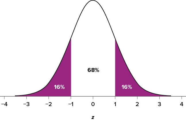
An important property to point out here is that, by virtue of the fact that the total area under the curve of a distribution is always equal to 1.0 (see section on Normal Distributions at the beginning of this chapter), these areas under the curve can be added together or subtracted from 1 to find the proportion in other areas. For example, we know that the area between z = −1.0 and z = 1.0 (i.e., within one standard deviation of the mean) contains 68% of the area under the curve, which can be represented in decimal form as .6800. (To change a percentage to a decimal, simply move the decimal point 2 places to the left.) Because the total area under the curve is equal to 1.0, that means that the proportion of the area outside z = −1.0 and z = 1.0 is equal to 1.0 − .6800 = .3200 or 32% (see Figure 4.3). This area is called the area in the tails of the distribution. Because this area is split between two tails and because the normal distribution is symmetrical, each tail has exactly one-half, or 16%, of the area under the curve.

We will have much more to say about this concept in the coming chapters. As it turns out, this is a quite powerful idea that enables us to make statements about how likely an outcome is and what that means for research questions we would like to answer and hypotheses we would like to test. But first, we need to make a brief foray into some ideas about probability in Chapter 5.

Exercises

1. What are the two pieces of information contained in a z score?
2. A z score takes a raw score and standardizes it into units of .
3. Assume the following five scores represent a sample: 2, 3, 5, 5, 6. Transform these scores into z scores.
4. True or false:
   1. All normal distributions are symmetrical.
   2. All normal distributions have a mean of 1.0.
   3. All normal distributions have a standard deviation of 1.0.
   4. The total area under the curve of all normal distributions is equal to 1.
5. Interpret the location, direction, and distance (near or far) of the following z scores:
   1. −2.00
   2. 1.25
   3. 3.50
   4. −0.34
6. Transform the following z scores into a distribution with a mean of 10 and standard deviation of 2: −1.75, 2.20, 1.65, −0.95
7. Calculate z scores for the following raw scores taken from a population with a mean of 100 and standard deviation of 16: 112, 109, 56, 88, 135, 99
8. What does a z score of 0.00 represent?
9. For a distribution with a standard deviation of 20, find z scores that correspond to:
   1. One-half of a standard deviation below the mean
   2. 5 points above the mean
   3. Three standard deviations above the mean
   4. 22 points below the mean
10. Calculate the raw score for the following z scores from a distribution with a mean of 15 and standard deviation of 3:
    1. 4.0
    2. 2.2
    3. −1.3
    4. 0.46