10 Chapter 10: Independent Samples

We have seen how to compare a single mean against a given value and how to utilize difference scores to look for meaningful, consistent change via a single mean difference. Now, we will learn how to compare two separate means from groups that do not overlap to see if there is a difference between them. The process of testing hypotheses about two means is exactly the same as it is for testing hypotheses about a single mean, and the logical structure of the formulas is the same as well. However, we will be adding a few extra steps this time to account for the fact that our data are coming from different sources.

Difference of Means

In Chapter 9, we learned about mean differences, that is, the average value of difference scores. Those difference scores came from one group and two time points (or two perspectives). Now, we will deal with the difference of the means, that is, the average values of separate groups that are represented by separate descriptive statistics. This analysis involves two groups and one time point. As with all of our other tests as well, both of these analyses are concerned with a single variable.

It is very important to keep these two tests separate and understand the distinctions between them because they assess very different questions and require different approaches to the data. When in doubt, think about how the data were collected and where they came from. If they came from two time points with the same people (sometimes referred to as “longitudinal” data), you know you are working with two data points from the same participant (the measurement was repeated) and will use a related samples t test (see Chapter 9). If it came from a single time point that used separate groups, you need to look at the nature of those groups and decide whether they are related. Can individuals in one group being meaningfully matched up with one and only one individual from the other group? For example, are they a romantic couple? If so, we call those data matched pairs and we use a related samples t test (Chapter 9). However, if there’s no logical or meaningful way to link individuals across groups, or if there is no overlap between the groups, then we say the groups are independent and use the independent samples t test, the subject of this chapter.

Research Questions about Independent Means

Many research ideas in the behavioral sciences and other areas of research are concerned with whether or not two means are the same or different. Logically, we therefore say that these research questions are concerned with group mean differences. That is, on average, do we expect a person from Group A to be higher or lower on some variable than a person from Group B. In any research design looking at group mean differences, there are some key criteria we must consider: the groups must be mutually exclusive (i.e., you can only be part of one group at any given time), and the groups have to be measured on the same variable (i.e., you can’t compare personality in one group to reaction time in another group since those values would not be the same anyway).

Let’s look at one of the most common and logical examples: testing a new medication. When a new medication is developed, the researchers who created it need to demonstrate that it effectively treats the symptoms they are trying to alleviate. The simplest design that will answer this question involves two groups: one group that receives the new medication (the “treatment” group) and one group that receives a placebo (the “control” group). Participants are randomly assigned to one of the two groups (remember that random assignment is the hallmark of a true experiment), and the researchers test the symptoms in each person in each group after they received either the medication or the placebo. They then calculate the average symptoms in each group and compare them to see if the treatment group did better (i.e., had fewer or less severe symptoms) than the control group.

In this example, we had two groups: treatment and control. Membership in these two groups was mutually exclusive—each individual participant received either the experimental medication or the placebo. No one in the experiment received both, so there was no overlap between the two groups. Additionally, each group could be measured on the same variable: symptoms related to the disease or ailment being treated. Because each group was measured on the same variable, the average scores in each group could be meaningfully compared. If the treatment was ineffective, we would expect that the average symptoms of someone receiving the treatment would be the same as the average symptoms of someone receiving the placebo (i.e., there is no difference between the groups). However, if the treatment was effective, we would expect fewer symptoms from the treatment group, leading to a lower group average.

Now let’s look at an example using groups that already exist. A common, and perhaps salient, question is how students feel about their job prospects after graduation. Suppose that we have narrowed our potential choice of college down to two universities and, in the course of trying to decide between the two, we come across a survey that has data from each university on how students at those universities feel about their future job prospects. As with our last example, we have two groups: University A and University B, and each participant is in only one of the two groups (assuming there are no transfer students who were somehow able to rate both universities). Because students at each university completed the same survey, they are measuring the same thing, so we can use a t test to compare the average perceptions of students at each university to see if they are the same. If they are the same, then we should continue looking for other things about each university to help us decide on where to go. But, if they are different, we can use that information in favor of the university with higher job prospects.

As we can see, the grouping variable we use for an independent samples t test can be a set of groups we create (as in the experimental medication example) or groups that already exist naturally (as in the university example). There are countless other examples of research questions relating to two group means, making the independent samples t test one of the most widely used analyses around.

Hypotheses and Decision Criteria

The process of testing hypotheses using an independent samples t test is the same as it was in the last three chapters, and it starts with stating our hypotheses and laying out the criteria we will use to test them.

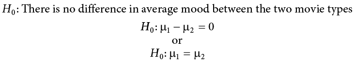
Our null hypothesis for an independent samples t test is the same as all others: there is no difference. The means of the two groups are the same under the null hypothesis, no matter how those groups were formed. Mathematically, this takes on two equivalent forms:

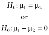
Both of these formulations of the null hypothesis tell us exactly the same thing: that the numerical value of the means is the same in both groups. This is more clear in the first formulation, but the second formulation also makes sense (any number minus itself is always zero) and helps us out a little when we get to the math of the test statistic. Either one is acceptable and you only need to report one. The English interpretation of both of them is also the same:

H0: There is no difference between the means of the two groups

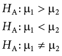
Our alternative hypotheses are also unchanged: we simply replace the equal sign (=) with one of the three inequalities (>, <, ≠):

or

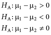
Whichever formulation you chose for the null hypothesis should be the one you use for the alternative hypothesis (be consistent), and the interpretation of them is always the same:

HA: There is a difference between the means of the two groups

Notice that we are now dealing with two means instead of just one, so it will be very important to keep track of which mean goes with which population and, by extension, which dataset and sample data. We use subscripts to differentiate between the populations, so make sure to keep track of which is which. If it is helpful, you can also use more descriptive subscripts. To use the experimental medication example:

Once we have our hypotheses laid out, we can set our criteria to test them using the same three pieces of information as before: significance level (), directionality (left, right, or two-tailed), and degrees of freedom, which for an independent samples t test are:

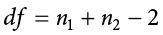
This looks different than before, but it is just adding the individual degrees of freedom from each group (n − 1) together. Notice that the sample sizes, n, also get subscripts so we can tell them apart.

For an independent samples t test, it is often the case that our two groups will have slightly different sample sizes, either due to chance or some characteristic of the groups themselves. Generally, this is not an issue, so long as one group is not massively larger than the other group. What is of greater concern is keeping track of which is which using the subscripts.

Independent Samples t Statistic

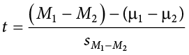
The test statistic for our independent samples t test takes on the same logical structure and format as our other t tests: our observed effect minus our null hypothesis value, all divided by the standard error:

This looks like more work to calculate, but remember that our null hypothesis states that the quantity 1 − 2 = 0, so we can drop that out of the equation and are left with:

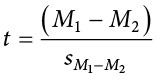
Our standard error in the denomination is still standard deviation (s) with a subscript denoting what it is the standard error of. Because we are dealing with the difference between two separate means, rather than a single mean or single mean of difference scores, we put both means in the subscript. Calculating our standard error, as we will see next, is where the biggest differences between this t test and other t tests appears. However, once we do calculate it and use it in our test statistic, everything else goes back to normal. Our decision criteria are still comparing our obtained test statistic to our critical value, and our interpretation based on whether or not we reject the null hypothesis is unchanged as well.

Standard Error and Pooled Variance

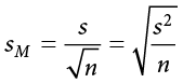
Recall that the standard error is the average distance between any given sample mean and the center of its corresponding sampling distribution, and it is a function of the standard deviation of the population (either given or estimated) and the sample size. This definition and interpretation hold true for our independent samples t test as well, but because we are working with two samples drawn from two populations, we have to first combine their estimates of standard deviation—or, more accurately, their estimates of variance—into a single value that we can then use to calculate our standard error.

The combined estimate of variance using the information from each sample is called the pooled variance and is denoted ; the subscript p serves as a reminder indicating that it is the pooled variance. The term “pooled variance” is a literal name because we are simply pooling or combining the information on variance—the sum of squares and degrees of freedom—from both of our samples into a single number. The result is a weighted average of the observed sample variances, the weight for each being determined by the sample size, and will always fall between the two observed variances. The computational formula for the pooled variance is:

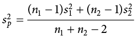
This formula can look daunting at first, but it is in fact just a weighted average. Even more conveniently, some simple algebra can be employed to greatly reduce the complexity of the calculation. The simpler and more appropriate formula to use when calculating pooled variance is:

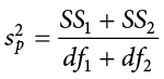
Using this formula, it’s very simple to see that we are just adding together the same pieces of information we have been calculating since Chapter 3. Thus, when we use this formula, the pooled variance is not nearly as intimidating as it might have originally seemed.

Once we have our pooled variance calculated, we can drop it into the equation for our standard error:

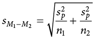
Once again, although this formula may seem different than it was before, in reality it is just a different way of writing the same thing. An alternative but mathematically equivalent way of writing our old standard error is:

Looking at that, we can now see that, once again, we are simply adding together two pieces of information—no new logic or interpretation required. Once the standard error is calculated, it goes in the denominator of our test statistic, as shown above and as was the case in all previous chapters. Thus, the only additional step to calculating an independent samples t statistic is computing the pooled variance. Let’s see an example in action.

Example Movies and Mood

We are interested in whether the type of movie someone sees at the theater affects their mood when they leave. We decide to ask people about their mood as they leave one of two movies: a comedy (Group 1, n = 35) or a horror film (Group 2, n = 29). Our data are coded so that higher scores indicate a more positive mood. We have good reason to believe that people leaving the comedy will be in a better mood, so we use a one-tailed test at a = .05 to test our hypothesis.

Step 1: State the Hypotheses

As always, we start with hypotheses:

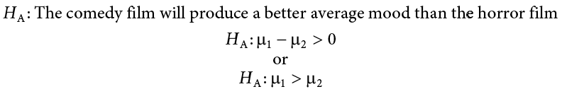
Notice that in the first formulation of the alternative hypothesis we say that the first mean minus the second mean will be greater than zero. This is based on how we code the data (higher is better), so we suspect that the mean of the first group will be higher. Thus, we will have a larger number minus a smaller number, which will be greater than zero. Be sure to pay attention to which group is which and how your data are coded (higher is almost always used as better outcomes) to make sure your hypothesis makes sense!

Step 2: Find the Critical Values

Just like before, we will need critical values, which come from our t table. In this example, we have a one-tailed test at a = .05 and expect a positive answer (because we expect the difference between the means to be greater than zero). Our degrees of freedom for our independent samples t test is just the degrees of freedom from each group added together: 35 + 29 − 2 = 62. From our t table, we find that our critical value is t* = 1.671. Note that because 62 does not appear on the table, we use the next lowest value, which in this case is 60.

Step 3: Compute the Test Statistic and Effect Size

The data from our two groups are presented in the tables below. Table 10.1 shows the values for the Comedy group, and Table 10.2 shows the values for the Horror group. Values for both have already been placed in the sum of squares tables since we will need to use them for our further calculations. As always, the column on the left is our raw data.

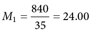
Using the sum of the first column for each table, we can calculate the mean for each group:

and

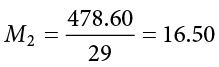
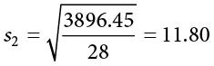
These values were used to calculate the middle rows of each table, which sum to zero as they should (the middle column for Group 2 sums to a very small value instead of zero due to rounding error—the exact mean is 16.50344827586207, but that’s far more than we need for our purposes). Squaring each of the deviation scores in the middle columns gives us the values in the third columns, which sum to our next important value: the sum of squares for each group: SS1 = 5061.60 and SS2 = 3896.45. These values have all been calculated and take on the same interpretation as they have since Chapter 3—no new computations yet. Before we move on to the pooled variance that will allow us to calculate standard error, let’s compute our standard deviation for each group; even though we will not use them in our calculation of the test statistic, they are still important descriptors of our data:

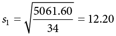
and

Now we can move on to our new calculation, the pooled variance, which is just the sums of squares that we calculated from our table and the degrees of freedom, which is just n − 1 for each group:

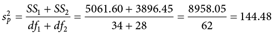
As you can see, if you follow the regular process of calculating standard deviation using the sum of squares table, finding the pooled variance is very easy. Now we can use that value to calculate our standard error, the last step before we can find our test statistic:

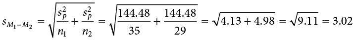
Finally, we can use our standard error and the means we calculated earlier to compute our test statistic. Because the null hypothesis value of 1 − 2 is 0.00, we will leave that portion out of the equation for simplicity:

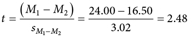
The process of calculating our obtained test statistic t = 2.48 followed the same sequence of steps as before: use raw data to compute the mean and sum of squares (this time for two groups instead of one), use the sum of squares and degrees of freedom to calculate standard error (this time using pooled variance instead of standard deviation), and use that standard error and the observed means to get t.

Effect Sizes and Confidence Intervals

We have seen in previous chapters that even a statistically significant effect needs to be interpreted along with an effect size to see if it is practically meaningful. We have also seen that our sample means, as a point estimate, are not perfect and would be better represented by a range of values that we call a confidence interval. As with all other topics, this is also true of our independent samples t tests.

Our effect size for the independent samples t test is still Cohen’s d, and it is still just our observed effect divided by the standard deviation. Remember that standard deviation is just the square root of the variance, and because we work with pooled variance in our test statistic, we will use the square root of the pooled variance as our denominator in the formula for Cohen’s d. This gives us:

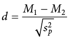
For our example above, we can calculate the effect size to be:

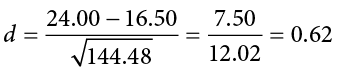
We interpret this using the same guidelines as before, so we would consider this a moderate or moderately large effect.

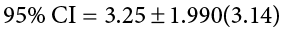
Our confidence intervals also take on the same form and interpretation as they have in the past. The value we are interested in is the difference between the two means, so our point estimate is the value of one mean minus the other, or . Just like before, this is our observed effect and is the same value as the one we place in the numerator of our test statistic. We calculate this value then place the margin of error—still our critical value multiplied by our standard error—above and below it. That is:

Because our hypothesis testing example used a one-tailed test, it would be inappropriate to calculate a confidence interval on those data (remember that we can only calculate a confidence interval for a two-tailed test because the interval extends in both directions). Let’s say we find summary statistics on the average life satisfaction of people from two different towns and want to create a confidence interval to see if the difference between the two might actually be zero.

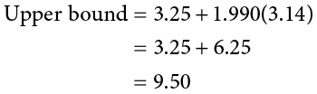
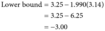
Our sample data are = 28.65, s1 = 12.40, n1 = 40 and = 25.40, s2 = 15.68, n2 = 42. At face value, it looks like the people from the first town have higher life satisfaction (28.65 vs. 25.40), but it will take a confidence interval (or complete hypothesis testing process) to see if that is true or just due to random chance. First, we want to calculate the difference between our sample means, which is 28.65 − 25.40 = 3.25. Next, we need a critical value from our t table. If we want to test at the normal 95% level of confidence, then our sample sizes will yield degrees of freedom equal to 40 + 42 − 2 = 80. From our table, that gives us a critical value of t* = 1.990. Finally, we need our standard error. Recall that our standard error for an independent samples t test uses pooled variance, which requires the sum of squares and degrees of freedom. Up to this point, we have calculated the sum of squares using raw data, but in this situation, we do not have access to it. So, what are we to do?

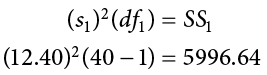
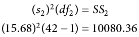
If we have summary data like standard deviation and sample size, it is very easy to calculate the pooled variance, and the key lies in rearranging the formulas to work backward through them. We need the sum of squares and degrees of freedom to calculate our pooled variance. Degrees of freedom is very simple: we just take the sample size minus 1.00 for each group. Getting the sum of squares is also easy: remember that variance is standard deviation squared and is the sum of squares divided by the degrees of freedom. That is:

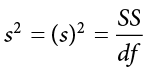
To get the sum of squares, we just multiply both sides of the above equation to get:

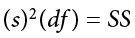
which is the squared standard deviation multiplied by the degrees of freedom (n − 1) equals the sum of squares.

Using our example data:

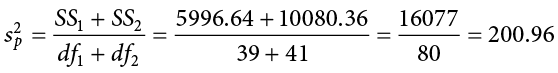
And thus our pooled variance equals:

And our standard error equals:

All of these steps are just slightly different ways of using the same formulas, numbers, and ideas we have worked with up to this point. Once we get out standard error, it’s time to build our confidence interval.

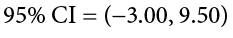
Our confidence interval, as always, represents a range of values that would be considered reasonable or plausible based on our observed data. In this instance, our interval (−3.00, 9.50) does contain zero. Thus, even though the means look a little bit different, it may very well be the case that the life satisfaction in both of these towns is the same. Proving otherwise would require more data.

Now we can move on to the final step of the hypothesis-testing procedure.

Step 4: Make the Decision

Our test statistic has a value of t = 2.48, and in Step 2 we found that the critical value is t* = 1.671. Because 2.48 > 1.671, we reject the null hypothesis:

Reject H0. Based on our sample data from people who watched different kinds of movies, we can say that the average mood after a comedy movie ( = 24.00, SD1 = 12.20) is better than the average mood after a horror movie ( = 16.50, SD2 = 11.80), t(62) = 2.48, p < .05, d = 0.62.

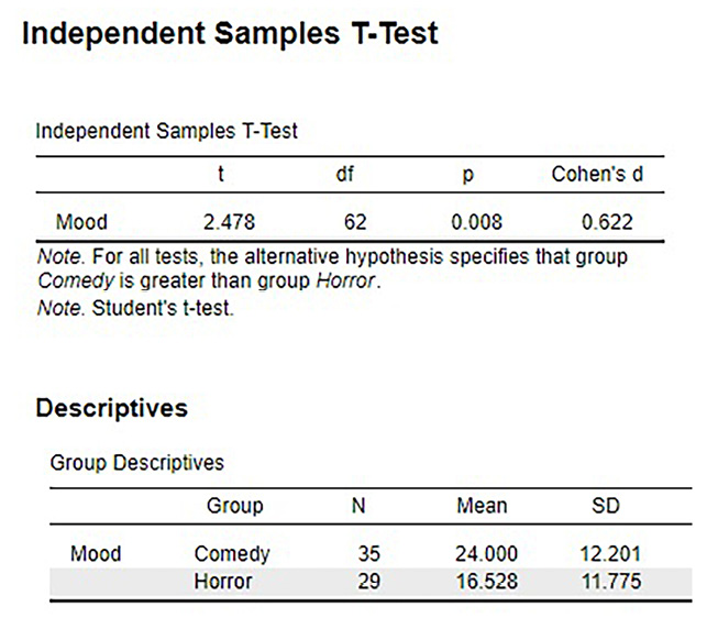
Figure 10.1 shows the output from JASP for this example.

Homogeneity of Variance

Before wrapping up the coverage of independent samples t tests, there is one other important topic to cover. Using the pooled variance to calculate the test statistic relies on an assumption known as homogeneity of variance. In statistics, an assumption is some characteristic that we assume is true about our data, and our ability to use our inferential statistics accurately and correctly relies on these assumptions being true. If these assumptions are not true, then our analyses are at best ineffective (e.g., low power to detect effects) and at worst inappropriate (e.g., too many Type I errors). A detailed coverage of assumptions is beyond the scope of this course, but it is important to know that they exist for all analyses.

For the current analysis, one important assumption is homogeneity of variance. This is fancy statistical talk for the idea that the true population variance for each group is the same and any difference in the observed sample variances is due to random chance. (If this sounds eerily similar to the idea of testing the null hypothesis that the true population means are equal, that’s because it is exactly the same!) This notion allows us to compute a single pooled variance that uses our easily calculated degrees of freedom. If the assumption is shown to not be true, then we have to use a very complicated formula to estimate the proper degrees of freedom. There are formal tests to assess whether or not this assumption is met, but we will not discuss them here.

Many statistical programs incorporate the test of homogeneity of variance automatically and can report the results of the analysis assuming it is true or assuming it has been violated. You can easily tell which is which by the degrees of freedom: the corrected degrees of freedom (which is used when the assumption of homogeneity of variance is violated) will have decimal places. Fortunately, the independent samples t test is very robust to violations of this assumption (an analysis is “robust” if it works well even when its assumptions are not met), which is why we do not bother going through the tedious work of testing and estimating new degrees of freedom by hand.

Exercises

1. What is meant by “the difference of the means” when talking about an independent samples t test? How does it differ from the “mean of the differences” in a related samples t test?
2. Describe three research questions that could be tested using an independent samples t test.
3. Calculate pooled variance from the following raw data:
   

   Group 1	Group 2
   16	4
   11	10
   9	15
   7	13
   5	12
   4	9
   12	8

4. Calculate the standard error from the following descriptive statistics.
   1. s1 = 24, s2 = 21, n1 = 36, n2 = 49
   2. s1 = 15.40, s2 = 14.80, n1 = 20, n2 = 23
   3. s1 = 12, s2 = 10, n1 = 25, n2 = 25
5. Determine whether to reject or fail to reject the null hypothesis in the following situations:
   1. t(40) = 2.49, a = .01, one-tailed test to the right
   2. = 64, = 54, n1 = 14, n2 = 12, = 9.75, a = .05, two-tailed test
   3. 95% CI: (0.50, 2.10)
6. A professor is interested in whether the type of software program used in a statistics lab affects how well students learn the material. The professor teaches the same lecture material to two classes but has one class use a point-and-click software program in lab and has the other class use a basic programming language. The professor collects final exam scores for students in each class. Conduct a hypothesis test to answer the research question.
   

   Point-and-Click	Programming
   83	86
   83	79
   63	100
   77	74
   86	70
   84	67
   78	83
   61	85
   65	74
   75	86
   100	87
   60	61
   90	76
   66	100
   54

7. A researcher wants to know if there is a difference in how busy someone is based on whether that person identifies as an early bird or a night owl. The researcher gathers data from people in each group, coding the data so that higher scores represent higher levels of being busy, and tests for a difference between the two at the .05 level of significance. Conduct a hypothesis test to answer the research question.
   

   Early Bird	Night Owl
   23	26
   28	10
   27	20
   33	19
   26	26
   30	18
   22	12
   25	25
   26

8. Lots of people claim that having a pet helps lower their stress level. Use the following summary data to test the claim that there is a lower average stress level among pet owners (Group 1) than among non-owners (Group 2) at the .05 level of significance.
   • = 16.25, = 20.95, s1 = 4.00, s2 = 5.10, n1 = 29, n2 = 25
9. Administrators at a university want to know if students in different majors are more or less extroverted than others. They provide you with descriptive statistics they have for English majors (coded as 1) and History majors (coded as 2) and ask you to create a confidence interval of the difference between them. Does this confidence interval suggest that the students from the majors differ?
   • = 3.78, = 2.23, s1 = 2.60, s2 = 1.15, n1 = 45, n2 = 40
10. Researchers want to know if people’s awareness of environmental issues varies as a function of where they live. Use the following summary data from two states, Alaska and Hawaii, to test for a difference.

• = 47.50, = 45.70, sH = 14.65, sA = 13.20, nH = 139, nA = 150

“Boyfriend” by Randall Munroe/xkcd.com is licensed under CC BY-NC 2.5.)