14 Chapter 14: Chi-Square
We come at last to our final topic: chi-square ( ). This test is a special form of analysis called a nonparametric test, so the structure of it will look a little bit different from what we have done so far. However, the logic of hypothesis testing remains unchanged. The purpose of chi-square is to understand the frequency distribution of a single categorical variable or find a relationship between two categorical variables, which is a frequently very useful way to look at our data.
Categories and Frequency Tables
Our data for the test are categorical—specifically nominal—variables. Recall from Unit 1 that nominal variables have no specified order and can only be described by their names and the frequencies with which they occur in the dataset. Thus, unlike the other variables we have tested, we cannot describe our data for the test using means and standard deviations. Instead, we will use frequencies tables.
Table 14.1 gives an example of a frequency table used for a test. The columns represent the different categories within our single variable, which in this example is pet preference. The test can assess as few as two categories, and there is no technical upper limit on how many categories can be included in our variable, although, as with ANOVA, having too many categories makes our computations long and our interpretation difficult. The final column in the table is the total number of observations, or  . The test assumes that each observation comes from only one person and that each person will provide only one observation, so our total observations will always equal our sample size.
There are two rows in this table. The first row gives the observed frequencies of each category from our dataset; in this example, 14 people reported preferring cats as pets, 17 people reported preferring dogs, and 5 people reported a different animal. The second row gives expected values; expected values are what would be found if each category had equal representation. The calculation for an expected value is:

where is the total number of people in our sample and C is the number of categories in our variable (also the number of columns in our table). The expected values correspond to the null hypothesis for tests: equal representation of categories. Our first of two tests, the test for goodness of fit, will assess how well our data lines up with, or deviates from, this assumption.
Test for Goodness of Fit
The test for goodness of fit assesses one categorical variable against a null hypothesis of equally sized frequencies. Equal frequency distributions are what we would expect to get if categorization was completely random. We could, in theory, also test against a specific distribution of category sizes if we have a good reason to. If we have information about how a population is distributed, we could compare our observed sample distribution to the expected values if the sample followed the same distribution as the population. For example, if we know that in the population of a small liberal arts college, 15% of students are international students, while 85% are domestic students, we would then calculate expected values for our sample using these percentages. In that case, we would be testing against the null hypothesis of 15% international students. This is less common, so we will not deal with more examples of this sort in this text.
Hypotheses
All tests, including the test for goodness of fit, are nonparametric tests. This means that there is no population parameter we are estimating or testing against; we are working only with our sample data. Because of this, there are no mathematical statements for hypotheses. This should make sense because the mathematical hypothesis statements were always about population parameters (e.g.,  ), so if we are nonparametric, we have no parameters and therefore no mathematical statements.
We do, however, still state our hypotheses verbally. For tests for goodness of fit, our null hypothesis is that there is an equal number of observations in each category. That is, there is no difference between the categories in how prevalent they are. Our alternative hypothesis says that the categories do differ in their frequency. We do not have specific directions or one-tailed tests for , matching our lack of mathematical statements.
Degrees of Freedom and the  Table
Table
Our degrees of freedom for the test are based on the number of categories we have in our variable, not on the number of people or observations like it was for our other tests. Luckily, they are still as simple to calculate:
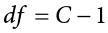
So for our pet preference example, we have 3 categories, thus we have 2 degrees of freedom. Our degrees of freedom, along with our significance level (still defaulted to a = .05) are used to find our critical values in the table, a portion of which is shown in Table 14.2. (The complete table can be found in Appendix E.) Because we do not have directional hypotheses for tests, we do not need to differentiate between critical values for one- or two-tailed tests. In fact, just like our F tests for regression and ANOVA, all tests are one-tailed tests.
Table 14.2. Critical Values for Chi-Square ( Table)
|
df |
Proportion in Critical Region |
||||
|
.1 |
.05 |
.02 |
.01 |
.005 |
|
|
1 |
2.706 |
3.841 |
5.024 |
6.635 |
7.879 |
|
2 |
4.605 |
5.991 |
7.378 |
9.210 |
10.597 |
|
3 |
6.251 |
7.815 |
9.348 |
11.345 |
12.838 |
|
4 |
7.779 |
9.488 |
11.143 |
13.277 |
14.860 |
|
5 |
9.236 |
11.070 |
12.833 |
15.086 |
16.750 |
|
6 |
10.645 |
12.592 |
14.449 |
16.812 |
18.548 |
|
7 |
12.017 |
14.067 |
16.013 |
18.475 |
20.278 |
|
8 |
13.362 |
15.507 |
17.535 |
20.090 |
21.955 |
|
9 |
14.684 |
16.919 |
19.023 |
21.666 |
23.589 |
|
10 |
15.987 |
18.307 |
20.483 |
23.209 |
25.188 |
 Statistic
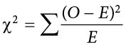
The calculations for our test statistic in tests combine our information from our observed frequencies (O) and our expected frequencies (E) for each level of our categorical variable. For each cell (category) we find the difference between the observed and expected values, square them, and divide by the expected values. We then sum this value across cells for our test statistic. This is shown in the formula:
For our pet preference data, we would have:

Notice that, for each cell’s calculation, the expected value in the numerator and the expected value in the denominator are the same value. Let’s now take a look at an example from start to finish.
Example Pineapple on Pizza
There is a very passionate and ongoing debate about whether pineapple should go on pizza. Being the objective, rational data analysts that we are, we will collect empirical data to see if we can settle this debate once and for all. We gather data from a group of adults, asking for a simple yes-or-no answer.
Step 1: State the Hypotheses
We start, as always, with our hypotheses. Our null hypothesis of no difference states that an equal number of people will say they do and do not like pineapple on pizza, and our alternative hypothesis will be that one side wins out over the other:


Step 2: Find the Critical Value
To avoid any potential bias in this crucial analysis, we will leave  at its typical level. We have two options in our data (Yes or No), which will give us two categories. Based on this, we will have 1 degree of freedom. From our table, we find a critical value of 3.84.
Step 3: Calculate the Test Statistic and Effect Size
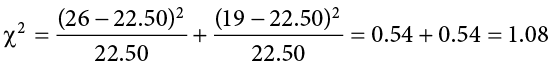
The results of the data collection are presented in Table 14.3. We had data from 45 people in all and 2 categories, so our expected values are E = 45/2 = 22.50.
We can use these to calculate our statistic:
Effect Size for 
Like all other significance tests, tests—both for goodness of fit and for independence—have effect sizes that can and should be calculated. There are many options for which effect size to use, and the ultimate decision is based on the type of data, the structure of your frequency or contingency table, and the types of conclusions you would like to draw. For the purpose of our introductory course, we will focus only on a single effect size that is simple and flexible: Cramer’s V.
Cramer’s V is a type of correlation coefficient that can be computed on categorical data. Like any other correlation coefficient (e.g., Pearson’s r), the cutoffs for small, medium, and large effect sizes of Cramer’s V are .10, .30, and .50, respectively. The calculation of Cramer’s V is very simple:
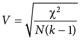
For this calculation, k is the smaller value of either R (the number of rows) or C (the number of columns). The numerator is simply the test statistic we calculate during Step 3 of the hypothesis-testing procedure. For our example, we had 2 rows and 3 columns, so k = 2:
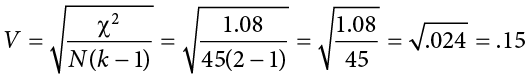
So the statistically significant relationship between our variables was moderately strong.
Step 4: Make the Decision
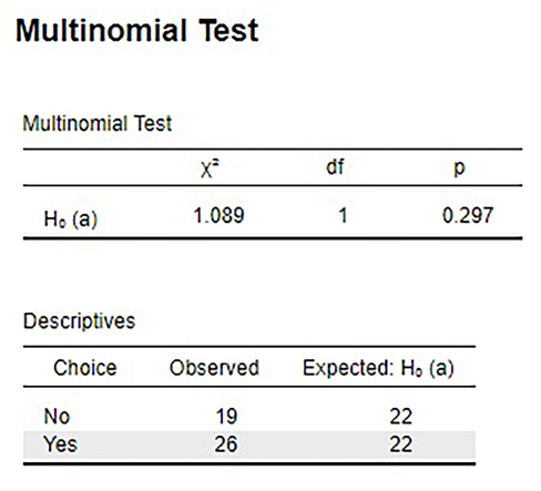
Our observed test statistic had a value of 1.08 and our critical value was 3.84. Our test statistic was smaller than our critical value, so we fail to reject the null hypothesis, and the debate rages on. Figure 14.1 shows the output from JASP for this example.
Figure 14.1. Output from JASP for the test for goodness of fit described in the Pineapple on Pizza example. The output provides the statistic (1.089), degrees of freedom (1) and the exact p value (.297, which is greater than .05). The output also provides the observed values and expected values (note that both expected values are 22.5, but decimals are not shown). Based on our sample of 45 people, there is no significant difference between the observed and expected values for preferring pineapple on pizza, (1, N = 45) = 1.089, p = .297. (“JASP chi-square goodness of fit” by Rupa G. Gordon/Judy Schmitt is licensed under CC BY-NC-SA 4.0.)
Contingency Tables for Two Variables
The test for goodness of fit is a useful tool for assessing a single categorical variable. However, what is more common is wanting to know if two categorical variables are related to one another. This type of analysis is similar to a correlation, the only difference being that we are working with nominal data, which violates the assumptions of traditional correlation coefficients. This is where the test for independence comes in handy.
As noted above, our only description for nominal data is frequency, so we will again present our observations in a frequency table. When we have two categorical variables, our frequency table is crossed. That is, each combination of levels from each categorical variable is presented. This type of frequency table is called a contingency table because it shows the frequency of each category in one variable, contingent upon the specific level of the other variable.
An example contingency table is shown in Table 14.4, which displays whether or not 168 college students watched college sports growing up (Yes/No) and whether the students’ final choice of which college to attend was influenced by the college’s sports teams (Yes, primary; Yes, somewhat; No).
In contrast to the frequency table for our test for goodness of fit, our contingency table does not contain expected values, only observed data. Within our table, wherever our rows and columns cross, we have a cell. A cell contains the frequency of observing its corresponding specific levels of each variable at the same time. The top left cell in Table 14.4 shows us that 47 people in our study watched college sports as a child and had college sports as their primary deciding factor in which college to attend.
Cells are numbered based on which row they are in (rows are numbered top to bottom) and which column they are in (columns are numbered left to right). We always name the cell using (R,C), with the row first and the column second. A quick and easy way to remember the order is that the brand RC Cola exists but CR Cola does not. Based on this convention, the top left cell containing our 47 participants who watched college sports as a child and had sports as a primary criteria is cell (1,1). Next to it, which has 26 people who watched college sports as a child but had sports only somewhat affect their decision, is cell (1,2), and so on. We only number the cells where our categories cross. We do not number our total cells, which have their own special name: marginal values.
Marginal values are the total values for a single category of one variable, added up across levels of the other variable. In Table 14.4, these marginal values have been made bold for ease of explanation, though this is not normally the case. We can see that, in total, 87 of our participants (47 + 26 + 14) watched college sports growing up and 81 (21 + 23 + 37) did not. The total of these two marginal values is 168, the total number of people in our study. Likewise, 68 people used sports as a primary criterion for deciding which college to attend, 50 considered it somewhat, and 50 did not consider it at all. The total of these marginal values is also 168, our total number of people. The marginal values for rows and columns will always both add up to the total number of participants, , in the study. If they do not, then a calculation error was made and you must go back and check your work.
Expected Values of Contingency Tables
Our expected values for contingency tables are based on the same logic as they were for frequency tables, but now we must incorporate information about how frequently each row and column was observed (the marginal values) and how many people were in the sample overall () to find what random chance would have made the frequencies out to be. Specifically:
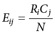
The subscripts i and j indicate which row and column, respectively, correspond to the cell we are calculating the expected frequency for, and the Ri and Cj are the row and column marginal values, respectively. is still the total sample size. Using the data from Table 14.4, we can calculate the expected frequency for cell (1,1), the college sport watchers who used sports at their primary criteria, to be:
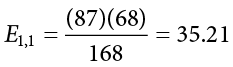
We can follow the same math to find all the expected values for this table:
|
Affected Decision |
|||||
|
Primary |
Somewhat |
No |
Total |
||
|
Watched as a child |
Yes |
35.21 |
25.38 |
26.41 |
87 |
|
No |
32.79 |
23.62 |
24.59 |
81 |
|
|
Total |
68 |
49 |
51 |
168 |
|
Notice that the marginal values still add up to the same totals as before. This is because the expected frequencies are just row and column averages simultaneously. Our total will also add up to the same value.
The observed and expected frequencies can be used to calculate the same statistic as we calculated for the test for goodness of fit. Before we get there, though, we should look at the hypotheses and degrees of freedom used for contingency tables.
Test for Independence
The test performed on contingency tables is known as the test for independence. In this analysis, we are looking to see if the values of each categorical variable (that is, the frequency of their levels) is related to or independent of the values of the other categorical variable. Because we are still doing a test, which is nonparametric, we still do not have mathematical versions of our hypotheses. The actual interpretations of the hypotheses are quite simple: the null hypothesis says that the variables are independent or not related, and the alternative hypothesis says that they are not independent or that they are related. Using this setup and the data provided in Table 14.4, let’s formally test for whether watching college sports as a child is related to using sports as a criteria for selecting a college to attend.
Example College Sports
We will follow the same four-step procedure as we have since Chapter 7.
Step 1: State the Hypotheses
Our null hypothesis of no difference will state that there is no relationship between our variables, and our alternative will state that our variables are related.


Step 2: Find the Critical Value
Our critical value will come from the same table that we used for the test for goodness of fit, but our degrees of freedom will change. Because we now have rows and columns (instead of just columns) our new degrees of freedom use information from both:
In our example:
Based on our 2 degrees of freedom, our critical value from our table is 5.991.
Step 3: Calculate the Test Statistic and Effect Size
The same formula for is used once again:
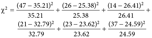

Step 4: Make the Decision
The final decision for our test of independence is still based on our observed value (20.31) and our critical value (5.991). Because our observed value is greater than our critical value, we can reject the null hypothesis.
Reject H0. Based on our data from 168 people, we can say that there is a statistically significant relationship between whether someone watches college sports growing up and the influence a college’s sports teams have on that person’s decision on which college to attend, and the effect size was moderate, (2, N = 168) = 20.31, p < .05, V < .348.
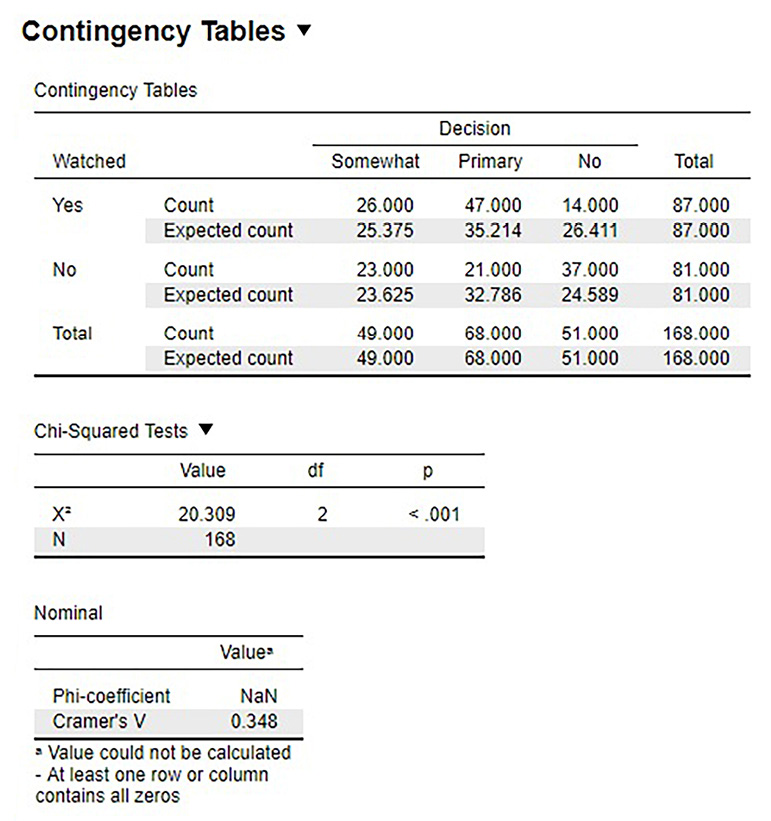
Figure 14.2 shows the output from JASP for this example.
Figure 14.2. Output from JASP for the test for independence described in the College Sports example. The output provides the statistic (20.309), degrees of freedom (2), and the p value of less than .001. The output also provides the observed count and expected count in the contingency table and Cramer’s V (.348) in the nominal table. Based on our data from 168 people, we can say that there is a statistically significant relationship between whether someone watches college sports growing up and the influence a college’s sports teams have on that person’s decision on which college to attend, (2, N = 168) = 20.31, p < .001, V = .348. (“JASP chi-square independence” by Rupa G. Gordon/Judy Schmitt is licensed under CC BY-NC-SA 4.0.)
Exercises
- What does a frequency table display? What does a contingency table display?
- What does a test for goodness of fit assess?
- How do expected frequencies relate to the null hypothesis?
- What does a test for independence assess?
- Compute the expected frequencies for the following contingency table:
Category A
Category B
Category C
22
38
Category D
16
14
- Test significance and find effect sizes for the following tests:
- N = 19, R = 3, C = 2, (2) = 7.89, a = .05
- N = 12, R = 2, C = 2, (1) = 3.12, a = .05
- N = 74, R = 3, C = 3, (4) = 28.41, a = .01
- N = 19, R = 3, C = 2,
- You hear a lot of people claim that The Empire Strikes Back is the best movie in the original Star Wars trilogy, and you decide to collect some data to demonstrate this empirically (pun intended). You ask 48 people which of the original movies they liked best; 8 said A New Hope was their favorite, 23 said The Empire Strikes Back was their favorite, and 17 said Return of the Jedi was their favorite. Perform a test on these data at the .05 level of significance.
- A pizza company wants to know if people order the same number of different toppings. They look at how many pepperoni, sausage, and cheese pizzas were ordered in the last week. Fill out the rest of the frequency table and test for a difference.
Pepperoni
Sausage
Cheese
Total
Observed
320
275
251
Expected
- A university administrator wants to know if there is a difference in proportions of students who go on to grad school across different majors. Use the data below to test whether there is a relationship between college major and going to grad school.
Major
Psychology
Business
Math
Graduate School
Yes
32
8
36
No
15
41
12
- A company you work for wants to make sure they are not discriminating against anyone in their promotion process. You have been asked to look across gender to see if there are differences in promotion rate (i.e., if gender and promotion rate are independent or not). The following data should be assessed at the normal level of significance:
Promoted in Last Two Years?
Yes
No
Gender
Women
8
5
Men
9
7
Answers to Odd-Numbered Exercises
1)
Frequency tables display observed category frequencies and (sometimes) expected category frequencies for a single categorical variable. Contingency tables display the frequency of observing people in crossed category levels for two categorical variables, and (sometimes) the marginal totals of each variable level.
3)
Expected values are what we would observe if the proportion of categories was completely random (i.e., no consistent difference other than chance), which is the same was what the null hypothesis predicts to be true.
5)
Observed:
|
Category A |
Category B |
Total |
|
|
Category C |
22 |
38 |
60 |
|
Category D |
16 |
14 |
30 |
|
Total |
38 |
52 |
90 |
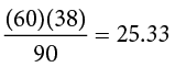
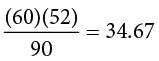
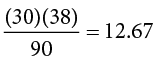
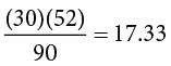
Expected:
|
Category A |
Category B |
Total |
|
|
Category C |
|
|
60 |
|
Category D |
|
|
30 |
|
Total |
38 |
52 |
90 |
7)
Step 1: H0: “There is no difference in preference for one movie,” HA: “There is a difference in how many people prefer one movie over the others.”
Step 2: Three categories (columns) gives df = 2,  = 5.991
Step 3: Based on the given frequencies:
|
New Hope |
Empire |
Jedi |
Total |
|
|
Observed |
8 |
23 |
17 |
48 |
|
Expected |
16 |
16 |
16 |
= 7.13. Since this is a statistically significant result, we should calculate an effect size:Cramer’s  , which is a moderate effect size
Step 4: Our obtained statistic is greater than our critical value, reject H0. Based on our sample of 48 people, there is a statistically significant difference in the proportion of people who prefer one Star Wars movie over the others, (2, N = 48) = 7.13, p < .05.
9)
Step 1: H0: “There is no relationship between college major and going to grad school,” HA: “Going to grad school is related to college major.”
Step 2: df = 2, = 5.991
Step 3: Based on the expected frequencies:
|
Major |
||||
|
Psychology |
Business |
Math |
||
|
Graduate School |
Yes |
24.81 |
25.86 |
25.33 |
|
No |
22.19 |
23.14 |
22.67 |
|
= 2.09 + 12.34 + 4.49 + 2.33 + 13.79 + 5.02 = 40.05Step 4: Obtained statistic is greater than the critical value, reject H0. Based on our data, there is a statistically significant relationship between college major and going to grad school, (2, N = 144) = 40.05, p < .05, V = .53, which is a large effect.
