5 Chapter 5: Probability

Probability can seem like a daunting topic for many students. In a mathematical statistics course this might be true, as the meaning and purpose of probability gets obscured and overwhelmed by equations and theory. In this chapter we will focus only on the principles and ideas necessary to lay the groundwork for future inferential statistics. We accomplish this by quickly tying the concepts of probability to what we already know about normal distributions and z scores.

What Is Probability?

When we speak of the probability of something happening, we are talking how likely it is that “thing” will happen based on the conditions present. For instance, what is the probability that it will rain? That is, how likely do we think it is that it will rain today under the circumstances or conditions today? To define or understand the conditions that might affect how likely it is to rain, we might look out the window and say, “It’s sunny outside, so it’s not very likely that it will rain today.” Stated using probability language: given that it is sunny outside, the probability of rain is low. “Given” is the word we use to state what the conditions are. As the conditions change, so does the probability. Thus, if it were cloudy and windy outside, we might say, “Given the current weather conditions, there is a high probability that it is going to rain.”

In these examples, we spoke about whether or not it is going to rain. Raining is an example of an event, which is the catch-all term we use to talk about any specific thing happening; it is a generic term that we specified to mean “rain” in exactly the same way that “conditions” is a generic term that we specified to mean “sunny” or “cloudy and windy.”

It should also be noted that the terms “low” and “high” are relative and vague, and they will likely be interpreted different by different people (in other words: given how vague the terminology was, the probability of different interpretations is high). Most of the time we try to use more precise language or, even better, numbers to represent the probability of our event. Regardless, the basic structure and logic of our statements are consistent with how we speak about probability using numbers and formulas.

Let’s look at a slightly deeper example. Say we have a regular, six-sided die (note that die is singular and dice is plural) and want to know how likely it is that we will roll a 1. That is, what is the probability of rolling a 1, given that the die is not weighted (which would introduce what we call a bias, though that is beyond the scope of this chapter). We could roll the die and see if it is a 1 or not, but that won’t tell us about the probability, it will only tell us a single result. We could also roll the die hundreds or thousands of times, recording each outcome and seeing what the final list looks like, but this is time consuming, and rolling a die that many times may lead down a dark path to gambling or, worse, playing Dungeons & Dragons. What we need is a simple equation that represents what we are looking for and what is possible.

To calculate the probability of an event, which here is defined as rolling a 1 on an unbiased die, we need to know two things: how many outcomes satisfy the criteria of our event (stated differently, how many outcomes would count as what we are looking for) and the total number of outcomes possible. In our example, only a single outcome, rolling a 1, will satisfy our criteria, and there are a total of six possible outcomes (rolling a 1, rolling a 2, rolling a 3, rolling a 4, rolling a 5, and rolling a 6). Thus, the probability of rolling a 1 on an unbiased die is 1 in 6 or 1/6. Put into an equation using generic terms, we get:

We can also use P() as shorthand for probability and A as shorthand for an event:

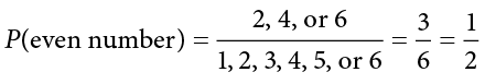
Using this equation, let’s now calculate the probability of rolling an even number on this die:

So we have a 50% chance of rolling an even number of this die. The principles laid out here operate under a certain set of conditions and can be elaborated into ideas that are complex yet powerful and elegant. However, such extensions are not necessary for a basic understanding of statistics, so we will end our discussion on the math of probability here. Now, let’s turn back to more familiar topics.

Probability in Graphs and Distributions

We will see shortly that the normal distribution is the key to how probability works for our purposes. To understand exactly how, let’s first look at a simple, intuitive example using pie charts.

Probability in Pie Charts

Recall that a pie chart represents how frequently a category was observed and that all slices of the pie chart add up to 100%, or 1. This means that if we randomly select an observation from the data used to create the pie chart, the probability of it taking on a specific value is exactly equal to the size of that category’s slice in the pie chart.

Take, for example, the pie chart in Figure 5.1 representing the favorite sports of 100 people. If you put this pie chart on a dart board and aimed blindly (assuming you are guaranteed to hit the board), the likelihood of hitting the slice for any given sport would be equal to the size of that slice. So, the probability of hitting the baseball slice is the highest at 36%. The probability is equal to the proportion of the chart taken up by that section.

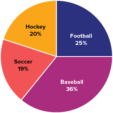
We can also add slices together. For instance, maybe we want to know the probability to finding someone whose favorite sport is usually played on grass. The outcomes that satisfy this criterion are baseball, football, and soccer. To get the probability, we simply add their slices together to see what proportion of the area of the pie chart is in that region: 36% + 25% + 20% = 81%. We can also add sections together even if they do not touch. If we want to know the likelihood that someone’s favorite sport is not called football somewhere in the world (i.e., baseball and hockey), we can add those slices even though they aren’t adjacent or contiguous in the chart itself: 36% + 20% = 56%. We are able to do all of this because (1) the size of the slice corresponds to the area of the chart taken up by that slice, (2) the percentage for a specific category can be represented as a decimal (this step was skipped for ease of explanation above), and (3) the total area of the chart is equal to 100% or 1.0, which makes the size of the slices interpretable.

Probability in Normal Distributions

If the language at the end of the last section sounded familiar, that’s because its exactly the language used in Chapter 4 to describe the normal distribution. Recall that the normal distribution has an area under its curve that is equal to 1 and that it can be split into sections by drawing a line through it that corresponds to a given z score. Because of this, we can interpret areas under the normal curve as probabilities that correspond to z scores.

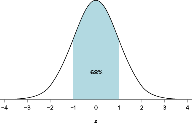
First, let’s look at the area between z = −1.00 and z = 1.00 presented in Figure 5.2. We were told earlier that this region contains 68% of the area under the curve. Thus, if we randomly chose a z score from all possible z scores, there is a 68% chance that it will be between z = −1.00 and z = 1.00 because those are the z scores that satisfy our criteria.

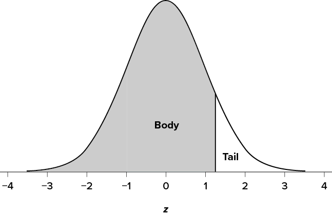
Just like a pie chart is broken up into slices by drawing lines through it, we can also draw a line through the normal distribution to split it into sections. Take a look at the normal distribution in Figure 5.3, which has a line drawn through it at z = 1.25. This line creates two sections of the distribution: the smaller section called the tail and the larger section called the body. Differentiating between the body and the tail does not depend on which side of the distribution the line is drawn. All that matters is the relative size of the pieces: bigger is always body.

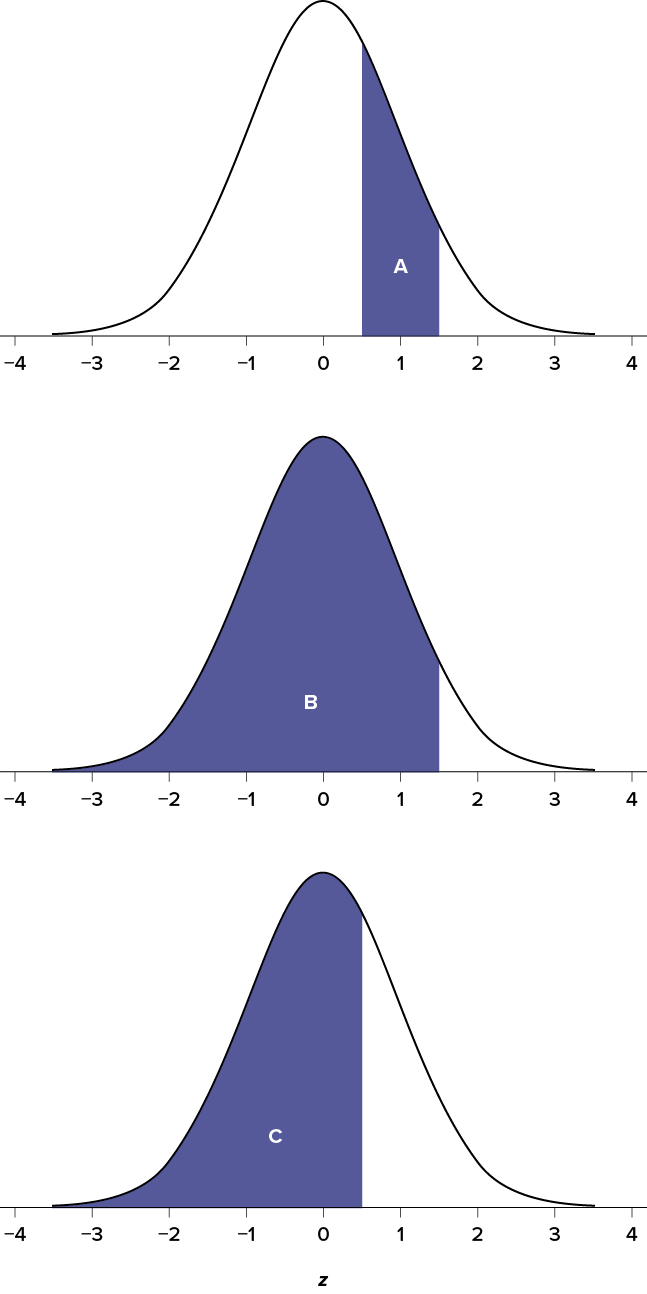
As you can see, we can break up the normal distribution into 3 pieces (lower tail, body, and upper tail) as in Figure 5.2 or into 2 pieces (body and tail) as in Figure 5.3. We can then find the proportion of the area in the body and tail based on where the line was drawn (i.e., at what z score). Mathematically, this is done using calculus. Fortunately, the exact values are given to you in the Standard Normal Distribution Table, also known at the z table. A portion of this table is shown in Figure 5.1. (The entire table appears in Appendix A.) Using the z values in the table (A), we can find the area under the normal curve in any body (B), tail (C), or combination of tails, as well as the proportion between z and the mean (D).

For example, suppose we want to find the area in the body for a z score of 1.62. As shown in Table 5.1, the row for 1.62 corresponds with a value of .9474 for the proportion in the body of the distribution. Thus, the odds of randomly selecting someone with a z score less than (to the left of) z = 1.62 is 94.74% because that is the proportion of the area taken up by values that satisfy our criteria.

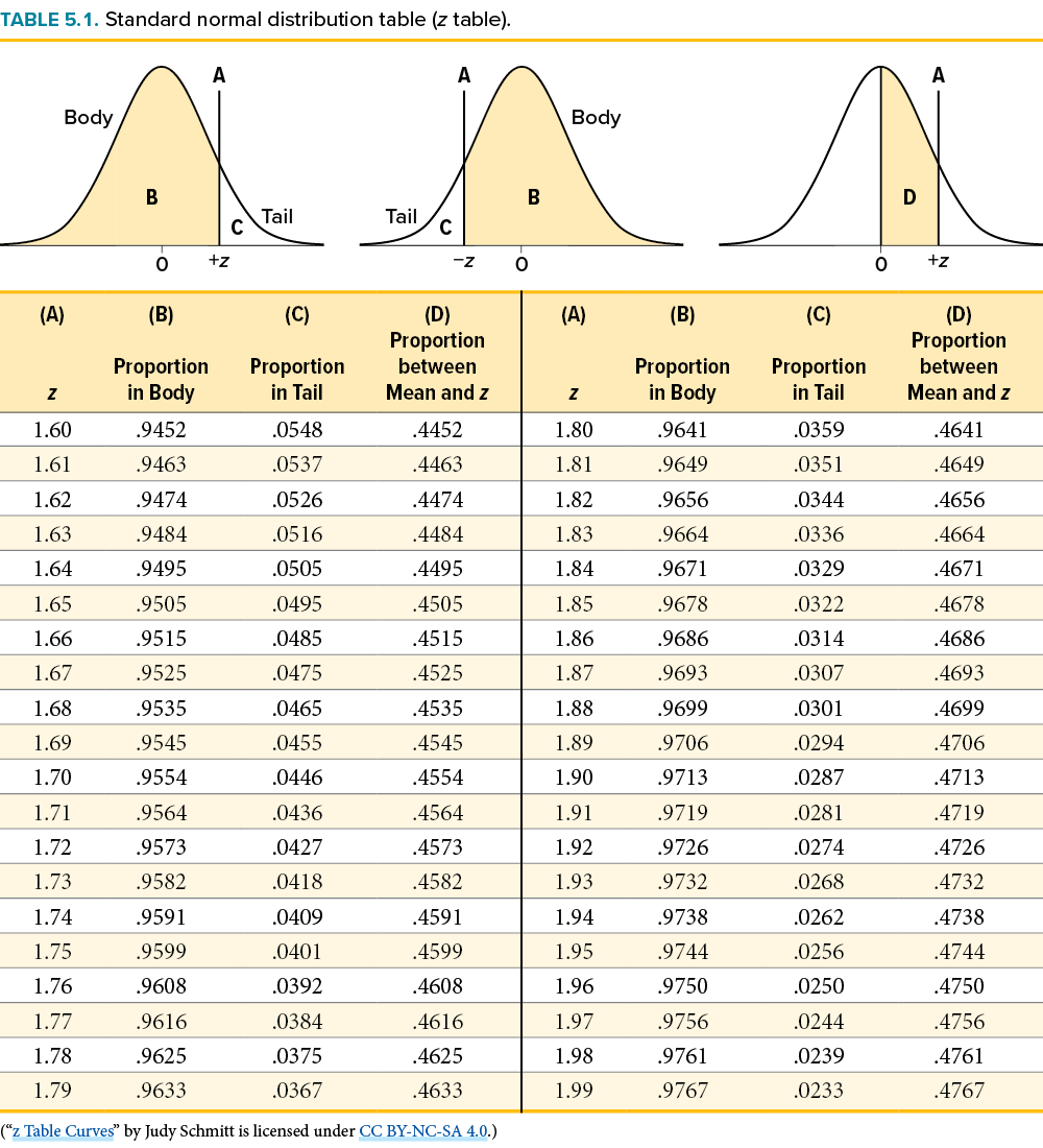
The z table only presents the area in the body for positive z scores because the normal distribution is symmetrical. Thus, the area in the body of z = 1.62 is equal to the area in the body for z = −1.62, though now—as illustrated in the middle distribution at the top of Table 5.1—the body will be the shaded area to the right of z. (When in doubt, drawing out your distribution and shading the area you need to find will always help.) Because the total area under the normal curve is always equal to 1.00, the area in the tail (Column C) is simply the area in the body (Column B) subtracted from 1.00 (1.00 − .9474 = .0526).

Let’s look at another example. This time, let’s find the area corresponding to z scores more extreme than z = −1.96 and z = 1.96. That is, let’s find the area in the tails of the distribution for values less than z = −1.96 (farther negative and therefore more extreme) and greater than z = 1.96 (farther positive and therefore more extreme). This region is illustrated in Figure 5.4.

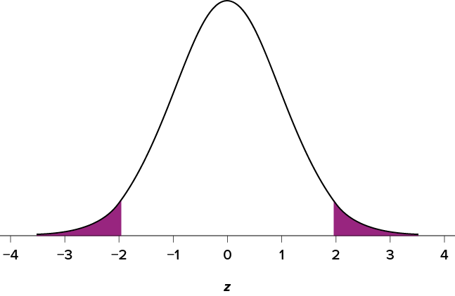
Let’s start with the tail for z = 1.96. If we go to the z table (Table 5.1) we will find that the area in the tail to the right of z = 1.96 is equal to .0250. Because the normal distribution is symmetrical, the area in the tail for z = −1.96 is the exact same value, .0250. Finally, to get the total area in the shaded region, we simply add the areas together to get .0500. Thus, there is a 5% chance of randomly getting a value more extreme than z = −1.96 or z = 1.96 (this particular value and region will become incredibly important in Unit 2).

Finally, we can find the area between two z scores by shading and subtracting. Figure 5.5 shows the area between z = 0.50 and z = 1.50. Because this is a subsection of a body (rather than just a body or a tail), we must first find the larger of the two bodies, in this case the body for z = 1.50, and subtract the smaller of the two bodies, or the body for z = 0.50. Aligning the distributions vertically, as in Figure 5.5, makes this clearer. From the complete z table in Appendix A, wee see that the area in the body for z = 1.50 is .9332, and the area in the body for z = 0.50 is .6915. Subtracting these gives us .9332 − .6915 = .2417.

Probability: The Bigger Picture

The concepts and ideas presented in this chapter are likely not intuitive at first. Probability is a tough topic for everyone, but the tools it gives us are incredibly powerful and enable us to do amazing things with data analysis. They are the heart of how inferential statistics work.

To summarize, the probability that an event happens is the number of outcomes that qualify as that event (i.e., the number of ways the event could happen) compared to the total number of outcomes (i.e., how many things are possible). This extends to graphs like a pie chart, where the biggest slices take up more of the area and are therefore more likely to be chosen at random. This idea then brings us back around to our normal distribution, which can also be broken up into regions or areas, each of which is bounded by one or two z scores and corresponds to all z scores in that region. The probability of randomly getting one of those z scores in the specified region can then be found on the Standard Normal Distribution Table. Thus, the larger the region, the more likely an event is, and vice versa. Because the tails of the distribution are, by definition, smaller and we go farther out into the tail, the likelihood or probability of finding a result out in the extremes becomes small.

Exercises

1. In your own words, what is probability?
2. There is a bag with 5 red blocks, 2 yellow blocks, and 4 blue blocks. If you reach in and grab one block without looking, what is the probability it is red?
3. Under a normal distribution, which of the following is more likely? (Note: this question can be answered without any calculations if you draw out the distributions and shade properly.)

   Getting a z score greater than z = 2.75
   Getting a z score less than z = −1.50

4. The heights of women in the United States are normally distributed with a mean of 63.7 inches and a standard deviation of 2.7 inches. If you randomly select a woman in the United States, what is the probability that she will be between 65 and 67 inches tall?
5. The heights of men in the United States are normally distributed with a mean of 69.1 inches and a standard deviation of 2.9 inches. What proportion of men are taller than 6 feet (72 inches)?
6. You know you need to score at least 82 points on the final exam to pass your class. After the final, you find out that the average score on the exam was 78 with a standard deviation of 7. How likely is it that you pass the class?
7. What proportion of the area under the normal curve is greater than z = 1.65?
8. Find the z score that bounds 25% of the lower tail of the distribution.
9. Find the z score that bounds the top 9% of the distribution.
10. In a distribution with a mean of 70 and standard deviation of 12, what proportion of scores are lower than 55?