1 Chapter 1: Introduction

This chapter provides an overview of statistics as a field of study and presents terminology that will be used throughout the course.

What Are Statistics?

Statistics include numerical facts and figures. For instance:

• The largest earthquake measured 9.2 on the Richter scale.f
• Men are at least 10 times more likely than women to commit murder.
• One in every eight South Africans is HIV positive.
• By the year 2050, there will be 12 people aged 65 and over for every new baby born.

The study of statistics involves math and relies upon calculations of numbers. But it also relies heavily on how the numbers are chosen and how the statistics are interpreted. For example, consider the following three scenarios and the interpretations based on the presented statistics. You will find that the numbers may be right, but the interpretation may be wrong. Try to identify a major flaw with each interpretation before we describe it.

1. A new advertisement for Ben & Jerry’s ice cream introduced in late May of last year resulted in a 30% increase in ice cream sales for the following three months. Thus, the advertisement was effective.
   Major flaw: Ice cream consumption generally increases in the months of June, July, and August regardless of advertisements. This effect is called a history effect and leads people to interpret outcomes as the result of one variable when another variable (in this case, one having to do with the passage of time) is actually responsible.
2. The more churches in a city, the more crime there is. Thus, churches lead to crime.
   Major flaw: Both increased churches and increased crime rates can be explained by larger populations. In bigger cities, there are both more churches and more crime. This problem, which we will discuss in more detail in Chapter 6, refers to the third-variable problem. Namely, a third variable can cause both situations; however, people erroneously believe that there is a causal relationship between the two primary variables rather than recognize that a third variable can cause both.
3. Seventy-five percent more interracial marriages are occurring this year than 25 years ago. Thus, our society accepts interracial marriages.
   Major flaw: We don’t have the information we need. What is the rate at which marriages are occurring? Suppose only 1% of marriages 25 years ago were interracial and so now 1.75% of marriages are interracial (1.75 is 75% higher than 1). But this latter number is hardly evidence suggesting the acceptability of interracial marriages. In addition, the statistic provided does not rule out the possibility that the number of interracial marriages has seen dramatic fluctuations over the years and this year is not the highest. Again, there is simply not enough information to understand fully the impact of the statistics.

As a whole, these examples show that statistics are not only facts and figures; they are something more than that. In the broadest sense, “statistics” refers to a range of techniques and procedures for analyzing, interpreting, displaying, and making decisions based on data.

Statistics is the language of science and data. The ability to understand and communicate using statistics enables researchers from different labs, different languages, and different fields to articulate to one another exactly what they have found in their work. It is an objective, precise, and powerful tool in science and in everyday life.

What a Statistics Course Is Not

Many psychology students dread the idea of taking a statistics course, and more than a few have changed majors upon learning that it is a requirement. That is because many students view statistics as a math class, which is actually not true. While many of you will not believe this or agree with it, statistics isn’t math.

Although math is a central component of it, statistics is a broader way of organizing, interpreting, and communicating information in an objective manner. Indeed, great care has been taken to eliminate as much math from this course as possible (students who do not believe this are welcome to ask the professor what matrix algebra is). Statistics is a way of viewing reality as it exists around us in a way that we otherwise could not.

Why Do We Study Statistics?

Virtually every student of the behavioral sciences takes some form of statistics class. This is because statistics is how we communicate in science. It serves as the link between a research idea and usable conclusions. Without statistics, we would be unable to interpret the massive amounts of information contained in data. Even small datasets contain hundreds—if not thousands—of numbers, each representing a specific observation we made. Without a way to organize these numbers into a more interpretable form, we would be lost, having wasted the time and money of our participants, ourselves, and the communities we serve.

Beyond its use in science, however, there is a more personal reason to study statistics. Like most people, you probably feel that it is important to “take control of your life.” But what does this mean? Partly, it means being able to properly evaluate the data and claims that bombard you every day. If you cannot distinguish good from faulty reasoning, then you are vulnerable to manipulation and to decisions that are not in your best interest. Statistics provides tools that you need in order to react intelligently to information you hear or read. In this sense, statistics is one of the most important things that you can study.

To be more specific, here are some claims that we have heard on several occasions. (We are not saying that each one of these claims is true!)

• Four out of five dentists recommend Dentine.
• Almost 85% of lung cancers in men and 45% in women are tobacco-related.
• Condoms are effective 94% of the time.
• People tend to be more persuasive when they look others directly in the eye and speak loudly and quickly.
• Women make 75 cents to every dollar a man makes when they work the same job.
• A surprising new study shows that eating egg whites can increase one’s life span.
• People predict that it is very unlikely there will ever be another baseball player with a batting average over 400.
• There is an 80% chance that in a room full of 30 people at least two people will share the same birthday.
• 79.48% of all statistics are made up on the spot.

All of these claims are statistical in character. We suspect that some of them sound familiar; if not, we bet that you have heard other claims like them. Notice how diverse the examples are. They come from psychology, health, law, sports, business, etc. Indeed, data and data interpretation show up in discourse from virtually every facet of contemporary life.

Statistics are often presented in an effort to add credibility to an argument or advice. You can see this by paying attention to television advertisements. Many of the numbers thrown about in this way do not represent careful statistical analysis. They can be misleading and push you into decisions that you might find cause to regret. For these reasons, learning about statistics is a long step toward taking control of your life. (It is not, of course, the only step needed to do so.) The purpose of this course, beyond preparing you for a career in psychology, is to help you learn statistical essentials. It will make you into an intelligent consumer of statistical claims.

You can take the first step right away. To be an intelligent consumer of statistics, your first reflex must be to question the statistics you encounter. The British Prime Minister Benjamin Disraeli is quoted by Mark Twain as having said, “There are three kinds of lies—lies, damned lies, and statistics.” This quote reminds us why it is so important to understand statistics. So let us invite you to reform your statistical habits from now on. No longer will you blindly accept numbers or findings. Instead, you will begin to think about the numbers, their sources, and most importantly, the procedures used to generate them.

The above section puts an emphasis on defending ourselves against fraudulent claims wrapped up as statistics, but let us look at a more positive note. Just as important as detecting the deceptive use of statistics is the appreciation of the proper use of statistics. You must also learn to recognize statistical evidence that supports a stated conclusion. Statistics are all around you, sometimes used well, sometimes not. We must learn how to distinguish the two cases. In doing so, statistics will likely be the course you use most in your day-to-day life, even if you do not ever run a formal analysis again.

Types of Data and How to Collect Them

In order to use statistics, we need data to analyze. Data come in an amazingly diverse range of formats, and each type gives us a unique type of information. In virtually any form, data represent the measured value of variables. A variable is simply a characteristic or feature of the thing we are interested in understanding. In psychology, we are interested in people, so we might get a group of people together and measure their levels of stress (one variable), anxiety (a second variable), and their physical health (a third variable). Once we have data on these three variables, we can use statistics to understand if and how they are related. Before we do so, we need to understand the nature of our data—what they represent and where they came from.

Types of Variables

When conducting research, experimenters often manipulate variables. For example, an experimenter might compare the effectiveness of four types of antidepressants. In this case, the variable is “type of antidepressant.” When a variable is manipulated by an experimenter, it is called an independent variable. The experiment seeks to determine the effect of the independent variable on relief from depression. In this example, relief from depression is called a dependent variable. In general, the independent variable is manipulated by the experimenter, and its effects on the dependent variable are measured.

Example #1: Can blueberries slow aging? A study indicates that antioxidants found in blueberries may slow down the process of aging. In this study, 19-month-old rats (equivalent to 60-year-old humans) were fed either their standard diet or a diet supplemented by either blueberry, strawberry, or spinach powder. After eight weeks, the rats were given memory and motor skills tests. Although all supplemented rats showed improvement, those supplemented with blueberry powder showed the most notable improvement.

1. What is the independent variable? (dietary supplement: none, blueberry, strawberry, and spinach)
2. What are the dependent variables? (memory test and motor skills test)

Example #2: Does beta-carotene protect against cancer? Beta-carotene supplements have been thought to protect against cancer. However, a study published in the Journal of the National Cancer Institute suggests this is false. The study was conducted with 39,000 women aged 45 and over. These women were randomly assigned to receive a beta-carotene supplement or a placebo, and their health was studied over their lifetime. Cancer rates for women taking the beta-carotene supplement did not differ systematically from the cancer rates of those women taking the placebo.

1. What is the independent variable? (supplements: beta-carotene or placebo)
2. What is the dependent variable? (occurrence of cancer)

Example #3: How bright is right? An automobile manufacturer wants to know how bright brake lights should be in order to minimize the time required for the driver of a following car to realize that the car in front is stopping and to hit the brakes.

1. What is the independent variable? (brightness of brake lights)
2. What is the dependent variable? (time to hit brakes)

Levels of an Independent Variable

If an experiment compares an experimental treatment with a control treatment, then the independent variable (type of treatment) has two levels: experimental and control. If an experiment were comparing five types of diets, then the independent variable (type of diet) would have 5 levels. In general, the number of levels of an independent variable is the number of experimental conditions.

Qualitative and Quantitative Variables

An important distinction between variables is between qualitative variables and quantitative variables. Qualitative variables are those that express a qualitative attribute such as hair color, eye color, religion, favorite movie, gender, and so on. The values of a qualitative variable do not imply a numerical ordering. Values of the variable “religion” differ qualitatively; no ordering of religions is implied. Qualitative variables are sometimes referred to as categorical or nominal variables. Quantitative variables are those variables that are measured in terms of numbers. Some examples of quantitative variables are height, weight, and shoe size.

In the study on the effect of diet discussed previously, the independent variable was type of supplement: none, strawberry, blueberry, and spinach. The variable “type of supplement” is a qualitative variable; there is nothing quantitative about it. In contrast, the dependent variable “memory test” is a quantitative variable since memory performance was measured on a quantitative scale (number correct).

Discrete and Continuous Variables

Variables such as number of children in a household are called discrete variables since the possible scores are discrete points on the scale. For example, a household could have three children or six children, but not 4.53 children. Other variables such as time to respond to a question are continuous variables since the scale is continuous and not made up of discrete steps. The response time could be 1.64 seconds, or it could be 1.64237123922121 seconds. Of course, the practicalities of measurement preclude most measured variables from being truly continuous.

Levels of Measurement

Before we can conduct a statistical analysis, we need to measure our dependent variable. Exactly how the measurement is carried out depends on the type of variable involved in the analysis. Different types are measured differently. To measure the time taken to respond to a stimulus, you might use a stop watch. Stop watches are of no use, of course, when it comes to measuring someone’s attitude toward a political candidate. A rating scale is more appropriate in this case (with labels like “very favorable,” “somewhat favorable,” etc.). For a dependent variable such as favorite color, you can simply note the color-word (like “red”) that the subject offers.

Although procedures for measurement differ in many ways, they can be classified using a few fundamental categories. In a given category, all of the procedures share some properties that are important for you to know about. The categories are called “scale types,” or just “scales,” and are described in this section.

Nominal Scales

When measuring using a nominal scale, one simply names or categorizes responses. Gender, handedness, favorite color, and religion are examples of variables measured on a nominal scale. The essential point about nominal scales is that they do not imply any ordering among the responses. For example, when classifying people according to their favorite color, there is no sense in which green is placed “ahead of” blue. Responses are merely categorized. Nominal scales embody the lowest level of measurement.

Ordinal Scales

A researcher wishing to measure consumers’ satisfaction with their microwave ovens might ask them to specify their feelings as either “very dissatisfied,” “somewhat dissatisfied,” “somewhat satisfied,” or “very satisfied.” The items in this scale are ordered, ranging from least to most satisfied. This is what distinguishes ordinal from nominal scales. Unlike a nominal scale, an ordinal scale allows a comparison of the degree to which two subjects possess the dependent variable. For example, our satisfaction ordering makes it meaningful to assert that one person is more satisfied than another with their microwave oven. Such an assertion reflects the first person’s use of a verbal label that comes later in the list than the label chosen by the second person.

On the other hand, ordinal scales fail to capture important information that will be present in the other scales we examine. In particular, the difference between two levels of an ordinal scale cannot be assumed to be the same as the difference between two other levels. In our satisfaction scale, for example, the difference between the responses “very dissatisfied” and “somewhat dissatisfied” is probably not equivalent to the difference between “somewhat dissatisfied” and “somewhat satisfied.” Nothing in our measurement procedure allows us to determine whether the two differences reflect the same difference in psychological satisfaction. Statisticians express this point by saying that the differences between adjacent scale values do not necessarily represent equal intervals on the underlying scale giving rise to the measurements. (In our case, the underlying scale is the true feeling of satisfaction, which we are trying to measure.)

What if the researcher had measured satisfaction by asking consumers to indicate their level of satisfaction by choosing a number from 1 to 4? Would the difference between the responses of 1 and 2 necessarily reflect the same difference in satisfaction as the difference between the responses 2 and 3? The answer is no. Changing the response format to numbers does not change the meaning of the scale. We still are in no position to assert that the mental step from 1 to 2 (for example) is the same as the mental step from 3 to 4.

Interval Scales

An interval scale is a numerical scale in which intervals have the same interpretation throughout. As an example, consider the Fahrenheit scale of temperature. The difference between 30 degrees and 40 degrees represents the same temperature difference as the difference between 80 degrees and 90 degrees. This is because each 10-degree interval has the same physical meaning (in terms of the kinetic energy of molecules).

Interval scales are not perfect, however. In particular, they do not have a true zero point even if one of the scaled values happens to carry the name “zero.” The Fahrenheit scale illustrates the issue. Zero degrees Fahrenheit does not represent the complete absence of temperature (i.e., the absence of any molecular kinetic energy). In reality, the label “zero” is applied to its temperature for quite accidental reasons connected to the history of temperature measurement. Since an interval scale has no true zero point, it does not make sense to compute ratios of temperatures. For example, there is no sense in which the ratio of 40 to 20 degrees Fahrenheit is the same as the ratio of 100 to 50 degrees; no interesting physical property is preserved across the two ratios. After all, if the “zero” label were applied at the temperature that Fahrenheit happens to label as 10 degrees, the two ratios would instead be 30 to 10 and 90 to 40, no longer the same! For this reason, it does not make sense to say that 80 degrees is “twice as hot” as 40 degrees. Such a claim would depend on an arbitrary decision about where to “start” the temperature scale, namely, what temperature to call zero (whereas the claim is intended to make a more fundamental assertion about the underlying physical reality).

Ratio Scales

The ratio scale of measurement is the most informative scale. It is an interval scale with the additional property that its zero position indicates the absence of the quantity being measured. You can think of a ratio scale as the three earlier scales rolled up in one. Like a nominal scale, it provides a name or category for each object (the numbers serve as labels). Like an ordinal scale, the objects are ordered (in terms of the ordering of the numbers). Like an interval scale, the same difference at two places on the scale has the same meaning. And in addition, the same ratio at two places on the scale also carries the same meaning.

The Fahrenheit scale for temperature has an arbitrary zero point and is therefore not a ratio scale. However, zero on the Kelvin scale is absolute zero. This makes the Kelvin scale a ratio scale. For example, if one temperature is twice as high as another as measured on the Kelvin scale, then it has twice the kinetic energy of the other temperature.

Another example of a ratio scale is the amount of money you have in your pocket right now (25 cents, 55 cents, etc.). Money is measured on a ratio scale because, in addition to having the properties of an interval scale, it has a true zero point: if you have zero money, this implies the absence of money. Since money has a true zero point, it makes sense to say that someone with 50 cents has twice as much money as someone with 25 cents (or that Bill Gates has a million times more money than you do).

What Level of Measurement Is Used for Psychological Variables?

Rating scales are used frequently in psychological research. For example, experimental subjects may be asked to rate their level of pain, how much they like a consumer product, their attitudes about capital punishment, or their confidence in an answer to a test question. Typically these ratings are made on a 5-point or a 7-point scale. These scales are ordinal scales since there is no assurance that a given difference represents the same thing across the range of the scale. For example, there is no way to be sure that a treatment that reduces pain from a rated pain level of 3 to a rated pain level of 2 represents the same level of relief as a treatment that reduces pain from a rated pain level of 7 to a rated pain level of 6.

In memory experiments, the dependent variable is often the number of items correctly recalled. What scale of measurement is this? You could reasonably argue that it is a ratio scale. First, there is a true zero point; some subjects may get no items correct at all. Moreover, a difference of one represents a difference of one item recalled across the entire scale. It is certainly valid to say that someone who recalled 12 items recalled twice as many items as someone who recalled only 6 items.

But number-of-items recalled is a more complicated case than it appears at first. Consider the following example in which subjects are asked to remember as many items as possible from a list of ten. Assume that (a) there are five easy items and five difficult items, (b) half of the subjects are able to recall all the easy items and different numbers of difficult items, whereas (c) the other half of the subjects are unable to recall any of the difficult items but they do remember different numbers of easy items. Some sample data are shown in the following table.

Subject	Easy Items					Difficult Items					Score
Subject A	0	0	1	1	0	0	0	0	0	0	2
Subject B	1	0	1	1	0	0	0	0	0	0	3
Subject C	1	1	1	1	1	1	1	0	0	0	7
Subject D	1	1	1	1	1	0	1	1	0	1	8

Let’s compare (i) the difference between Subject A’s score of 2 and Subject B’s score of 3 and (ii) the difference between Subject C’s score of 7 and Subject D’s score of 8. The former difference is a difference of one easy item; the latter difference is a difference of one difficult item. Do these two differences necessarily signify the same difference in memory? We are inclined to respond “No” to this question since only a little more memory may be needed to retain the additional easy item whereas a lot more memory may be needed to retain the additional hard item. The general point is that it is often inappropriate to consider psychological measurement scales as either interval or ratio.

Consequences of Level of Measurement

Why are we so interested in the type of scale that measures a dependent variable? The crux of the matter is the relationship between the variable’s level of measurement and the statistics that can be meaningfully computed with that variable. For example, consider a hypothetical study in which five children are asked to choose their favorite color from blue, red, yellow, green, and purple. The researcher codes the results as follows:

Color	Code
Blue	1
Red	2
Yellow	3
Green	4
Purple	5

This means that if a child said her favorite color was “Red,” then the choice was coded as “2,” if the child said her favorite color was “Purple,” then the response was coded as 5, and so forth. Consider the following hypothetical data:

Subject	Color	Code
Subject 1	Blue	1
Subject 2	Blue	1
Subject 3	Green	4
Subject 4	Green	4
Subject 5	Purple	5

Each code is a number, so nothing prevents us from computing the average code assigned to the children. The average happens to be 3, but you can see that it would be senseless to conclude that the average favorite color is yellow (the color with a code of 3). Such nonsense arises because favorite color is a nominal scale, and taking the average of its numerical labels is like counting the number of letters in the name of a snake to see how long the beast is.

Does it make sense to compute the mean of numbers measured on an ordinal scale? This is a difficult question, one that statisticians have debated for decades. The prevailing (but by no means unanimous) opinion of statisticians is that for almost all practical situations, the mean of an ordinally measured variable is a meaningful statistic. However, there are extreme situations in which computing the mean of an ordinally measured variable can be very misleading.

Collecting Data

We are usually interested in understanding a specific group of people. This group is known as the population of interest, or simply the population. The population is the collection of all people who have some characteristic in common; it can be as broad as “all people” if we have a very general research question about human psychology, or it can be extremely narrow, such as “all freshmen psychology majors at Midwestern public universities” if we have a specific group in mind.

Populations and Samples

In statistics, we often rely on a sample—that is, a small subset of a larger set of data—to draw inferences about the larger set. The larger set is known as the population from which the sample is drawn.

Example #1: You have been hired by the National Election Commission to examine how the American people feel about the fairness of the voting procedures in the U.S. Whom will you ask?

It is not practical to ask every single American how he or she feels about the fairness of the voting procedures. Instead, we query a relatively small number of Americans and draw inferences about the entire country from their responses. The Americans actually queried constitute our sample of the larger population of all Americans.

A sample is typically a small subset of the population. In the case of voting attitudes, we would sample a few thousand Americans drawn from the hundreds of millions that make up the country. In choosing a sample, it is therefore crucial that it not over-represent one kind of citizen at the expense of others. For example, something would be wrong with our sample if it happened to be made up entirely of Florida residents. If the sample held only Floridians, it could not be used to infer the attitudes of other Americans. The same problem would arise if the sample were comprised only of Republicans. Inferences from statistics are based on the assumption that sampling is representative of the population. If the sample is not representative, then the possibility of sampling bias occurs. Sampling bias means that our conclusions apply only to our sample and are not generalizable to the full population.

Example #2: We are interested in examining how many math classes have been taken, on average, by current graduating seniors at American colleges and universities during their four years in school. Whereas our population in the last example included all U.S. citizens, now it involves just the graduating seniors throughout the country. This is still a large set since there are thousands of colleges and universities, each enrolling many students. (New York University, for example, enrolls 48,000 students.) It would be prohibitively costly to examine the transcript of every college senior. We therefore take a sample of college seniors and then make inferences to the entire population based on what we find. To make the sample, we might first choose some public and private colleges and universities across the United States. Then we might sample 50 students from each of these institutions. Suppose that the average number of math classes taken by the people in our sample were 3.2. We might speculate that 3.2 approximates the number we would find if we had the resources to examine every senior in the entire population. But we must be careful about the possibility that our sample is non-representative of the population. Perhaps we chose an overabundance of math majors, or chose too many technical institutions that have heavy math requirements. Such bad sampling makes our sample unrepresentative of the population of all seniors.

To solidify your understanding of sampling bias, consider the following examples. Try to identify the population and the sample, and then reflect on whether the sample is likely to yield the information desired.

Example #3: A substitute teacher wants to know how students in the class did on their last test. The teacher asks the ten students sitting in the front row to state their latest test score. He concludes from their report that the class did extremely well. What is the sample? What is the population? Can you identify any problems with choosing the sample in the way that the teacher did?

In Example #3, the population consists of all students in the class. The sample is made up of just the ten students sitting in the front row. The sample is not likely to be representative of the population. Those who sit in the front row tend to be more interested in the class and tend to perform higher on tests. Hence, the sample may perform at a higher level than the population.

Example #4: A coach is interested in how many cartwheels the average college freshmen at his university can do. Eight volunteers from the freshman class step forward. After observing their performance, the coach concludes that college freshmen can do an average of 16 cartwheels in a row without stopping.

In Example #4, the population is the class of all freshmen at the coach’s university. The sample is composed of the 8 volunteers. The sample is poorly chosen because volunteers are more likely to be able to do cartwheels than the average freshman; people who can’t do cartwheels probably did not volunteer! In the example, we are also not told of the gender of the volunteers. Were they all women, for example? That might affect the outcome, contributing to the non-representative nature of the sample (if the school is co-ed).

Simple Random Sampling

Researchers adopt a variety of sampling strategies. The most straightforward is simple random sampling. Such sampling requires every member of the population to have an equal chance of being selected into the sample. In addition, the selection of one member must be independent of the selection of every other member. That is, picking one member from the population must not increase or decrease the probability of picking any other member (relative to the others). In this sense, we can say that simple random sampling chooses a sample by pure chance. To check your understanding of simple random sampling, consider the following example. What is the population? What is the sample? Was the sample picked by simple random sampling? Is it biased?

Example #5: A research scientist is interested in studying the experiences of twins raised together versus those raised apart. She obtains a list of twins from the National Twin Registry, and selects two subsets of individuals for her study. First, she chooses all those in the registry whose last name begins with Z. Then she turns to all those whose last name begins with B. Because there are so many names that start with B, however, our researcher decides to incorporate only every other name into her sample. Finally, she mails out a survey and compares characteristics of twins raised apart versus together.

In Example #5, the population consists of all twins recorded in the National Twin Registry. It is important that the researcher only make statistical generalizations to the twins on this list, not to all twins in the nation or world. That is, the National Twin Registry may not be representative of all twins. Even if inferences are limited to the Registry, a number of problems affect the sampling procedure we described. For instance, choosing only twins whose last names begin with Z does not give every individual an equal chance of being selected into the sample. Moreover, such a procedure risks over-representing ethnic groups with many surnames that begin with Z. There are other reasons why choosing just the Zs may bias the sample.

Perhaps such people are more patient than average because they often find themselves at the end of the line! The same problem occurs with choosing twins whose last name begins with B. An additional problem for the Bs is that the every-other-one procedure disallowed adjacent names on the B part of the list from being both selected. Just this defect alone means the sample was not formed through simple random sampling.

Sample Size Matters

Recall that the definition of a random sample is a sample in which every member of the population has an equal chance of being selected. This means that the sampling procedure rather than the results of the procedure define what it means for a sample to be random. Random samples, especially if the sample size is small, are not necessarily representative of the entire population. For example, if a random sample of 20 subjects were taken from a population with an equal number of males and females, there would be a nontrivial probability (.06) that 70% or more of the sample would be female. Such a sample would not be representative, although it would be drawn randomly. Only a large sample size makes it likely that our sample is close to representative of the population. For this reason, inferential statistics take into account the sample size when generalizing results from samples to populations. In later chapters, you’ll see what kinds of mathematical techniques ensure this sensitivity to sample size.

More Complex Sampling

Sometimes it is not feasible to build a sample using simple random sampling. To see the problem, consider the fact that both Dallas and Houston competed to be hosts of the 2012 Olympics. Imagine that you had been hired to assess whether most Texans preferred Houston to Dallas as the host, or the reverse. Given the impracticality of obtaining the opinion of every single Texan, you had to construct a sample of the Texas population. But notice how difficult it would have been to proceed by simple random sampling. For example, how would you have contacted those individuals who didn’t vote and didn’t have a phone? Even among people you found in the telephone book, how could you have identified those who had just relocated to another state (and had no reason to inform you of their move)? What would you have done about the fact that since the beginning of the study, an additional 4,212 people took up residence in the state of Texas? As you can see, it is sometimes very difficult to develop a truly random procedure. For this reason, other kinds of sampling techniques have been devised. We now discuss two of them.

Stratified Sampling

Since simple random sampling often does not ensure a representative sample, a sampling method called stratified random sampling is sometimes used to make the sample more representative of the population. This method can be used if the population has a number of distinct “strata” or groups. In stratified sampling, you first identify members of your sample who belong to each group. Then you randomly sample from each of those subgroups in such a way that the sizes of the subgroups in the sample are proportional to their sizes in the population.

Let’s take an example: Suppose you were interested in views of capital punishment at an urban university. You have the time and resources to interview 200 students. The student body is diverse with respect to age; many older people work during the day and enroll in night courses (average age is 39), while younger students generally enroll in day classes (average age of 19). It is possible that night students have different views about capital punishment than day students. If 70% of the students were day students, it makes sense to ensure that 70% of the sample consisted of day students. Thus, your sample of 200 students would consist of 140 day students and 60 night students. The proportion of day students in the sample and in the population (the entire university) would be the same. Inferences to the entire population of students at the university would therefore be more secure.

Convenience Sampling

Not all sampling methods are perfect, and sometimes that’s okay. For example, if we are beginning research into a completely unstudied area, we may sometimes take some shortcuts to quickly gather data and get a general idea of how things work before fully investing a lot of time and money into well-designed research projects with proper sampling. This is known as convenience sampling, named for its ease of use. In limited cases, such as the one just described, convenience sampling is okay because we intend to follow up with a representative sample. Unfortunately, sometimes convenience sampling is used due only to its convenience without the intent of improving on it in future work.

Types of Research Designs

Research studies come in many forms, and, just like with the different types of data we have, different types of studies tell us different things. The choice of research design is determined by the research question and the logistics involved. Though a complete understanding of different research designs is the subject for at least one full class, if not more, a basic understanding of the principles is useful here. There are three types of research designs we will discuss: experimental, quasi-experimental, and non-experimental.

Experimental Designs

If we want to know if a change in one variable causes a change in another variable, we must use a true experiment. Experimental research is defined by the use of random assignment to treatment conditions and manipulation of the independent variable. To understand what this means, let’s look at an example:

A clinical researcher wants to know if a newly developed drug is effective in treating the flu. Working with collaborators at several local hospitals, she randomly samples 40 flu patients and randomly assigns each one to one of two conditions: Group A receives the new drug, and Group B receives a placebo. She measures the symptoms of all participants after one week to see if there is a difference in symptoms between the groups.

In the example, the independent variable is the drug treatment; we manipulate it into two levels: new drug or placebo. Without the researcher administering the drug (i.e., manipulating the independent variable), there would be no difference between the groups. Each person, after being randomly sampled to be in the research, was then randomly assigned to one of the two groups. That is, random sampling and random assignment are not the same thing and cannot be used interchangeably. For research to be a true experiment, random assignment must be used. For research to be representative of the population, random sampling must be used. The use of both techniques helps ensure that there are no systematic differences between the groups, thus eliminating the potential for sampling bias.

The dependent variable in the example is flu symptoms. Barring any other intervention, we would assume that people in both groups, on average, get better at roughly the same rate. Because there are no systematic differences between the two groups, if the researcher does find a difference in symptoms, she can confidently attribute it to the effectiveness of the new drug.

Quasi-Experimental Designs

Quasi-experimental research involves getting as close as possible to the conditions of a true experiment when we cannot meet all requirements. Specifically, a quasi-experiment involves manipulating the independent variable but not randomly assigning people to groups. There are several reasons this might be used. First, it may be unethical to deny potential treatment to someone if there is good reason to believe it will be effective and that the person would unduly suffer if they did not receive it. Alternatively, it may be impossible to randomly assign people to groups. Consider the following example:

A professor wants to test out a new teaching method to see if it improves student learning. Because he is teaching two sections of the same course, he decides to teach one section the traditional way and the other section using the new method. At the end of the semester, he compares the grades on the final for each class to see if there is a difference.

In this example, the professor has manipulated his teaching method, which is the independent variable, hoping to find a difference in student performance, the dependent variable. However, because students enroll in courses, he cannot randomly assign the students to a particular group, thus precluding using a true experiment to answer his research question. Because of this, we cannot know for sure that there are no systematic differences between the classes other than teaching style and therefore cannot determine causality.

Non-Experimental Designs

Finally, non-experimental research (sometimes called correlational research) involves observing things as they occur naturally and recording our observations as data. Consider this example:

A data scientist wants to know if there is a relationship between how conscientious a person is and whether that person is a good employee. She hopes to use this information to predict the job performance of future employees by measuring their personality when they are still job applicants. She randomly samples volunteer employees from several different companies, measuring their conscientiousness and having their bosses rate their performance on the job. She analyzes this data to find a relationship.

Here, it is not possible to manipulate conscientiousness, so the researcher must gather data from employees as they are in order to find a relationship between her variables. Although this technique cannot establish causality, it can still be quite useful. If the relationship between conscientiousness and job performance is consistent, then it doesn’t necessarily matter if conscientiousness causes good performance or if they are both caused by something else—she can still measure conscientiousness to predict future performance. Additionally, these studies have the benefit of reflecting reality as it actually exists since we as researchers do not change anything.

Types of Statistical Analyses

Now that we understand the nature of our data, let’s turn to the types of statistics we can use to interpret them. There are two types of statistics: descriptive and inferential.

Descriptive Statistics

Descriptive statistics are numbers that are used to summarize and describe data. The word “data” refers to the information that has been collected from an experiment, a survey, a historical record, etc. (By the way, data is plural. One piece of information is called a datum.) If we are analyzing birth certificates, for example, a descriptive statistic might be the percentage of certificates issued in New York State, or the average age of the mother. Any other number we choose to compute also counts as a descriptive statistic for the data from which the statistic is computed. Several descriptive statistics are often used at one time to give a full picture of the data.

Descriptive statistics are just descriptive. They do not involve generalizing beyond the data at hand. Generalizing from our data to another set of cases is the business of inferential statistics, which you’ll be studying in another section. Here we focus on (mere) descriptive statistics.

Some descriptive statistics are shown in Table 1.1. The table shows the average salaries for various occupations in the United States in 1999. Descriptive statistics like these offer insight into American society. It is interesting to note, for example, that we pay the people who educate our children and who protect our citizens a great deal less than we pay people who take care of our feet or our teeth.

For more descriptive statistics, consider Table 1.2. It shows the number of unmarried men per 100 unmarried women in U.S. metro areas in 1990. From this table we see that men outnumber women most in Jacksonville, North Carolina, and women outnumber men most in Sarasota, Florida. You can see that descriptive statistics can be useful if we are looking for an opposite-sex partner! (These data come from the Information Please Almanac.)

These descriptive statistics may make us ponder why the numbers are so disparate in these cities. One potential explanation, for instance, as to why there are more women in Florida than men may involve the fact that elderly individuals tend to move down to the Sarasota region and that women tend to outlive men. Thus, more women might live in Sarasota than men. However, in the absence of proper data, this is only speculation.

You probably know that descriptive statistics are central to the world of sports. Every sporting event produces numerous statistics, such as the shooting percentage of players on a basketball team. For the Olympic marathon (a foot race of 26.2 miles), we possess data that cover more than a century of competition. (The first modern Olympics took place in 1896.) Table 1.3 and Table 1.4 show the winning times for women and men, respectively. (Women have only been allowed to compete since 1984.)

Table 1.3. Women’s winning Olympic marathon times, 1984–2004.

Year	Winner	Country	Time
1984	Joan Benoit	United States	2:24:52
1988	Rosa Mota	Portugal	2:25:40
1992	Valentina Yegorova	Unified Team	2:32:41
1996	Fatuma Roba	Ethiopia	2:26:05
2000	Naoko Takahashi	Japan	2:23:14
2004	Mizuki Noguchi	Japan	2:26:20

Table 1.4. Men’s winning Olympic marathon times, 1896–2004.

Year	Winner	Country	Time
1896	Spyridon Louis	Greece	2:58:50
1900	Michel Théato	France	2:59:45
1904	Thomas Hicks	United States	3:28:53
1906	Billy Sherring	Canada	2:51:23
1908	Johnny Hayes	United States	2:55:18
1912	Kenneth McArthur	South Africa	2:36:54
1920	Hannes Kolehmainen	Finland	2:32:35
1924	Albin Stenroos	Finland	2:41:22
1928	Boughera El Ouafi	France	2:32:57
1932	Juan Carlos Zabala	Argentina	2:31:36
1936	Sohn Kee-chung	Japan	2:29:19
1948	Delfo Cabrera	Argentina	2:34:51
1952	Emil Zátopek	Czechoslovakia	2:23:03
1956	Alain Mimoun	France	2:25:00
1960	Abebe Bikila	Ethiopia	2:15:16
1964	Abebe Bikila	Ethiopia	2:12:11
1968	Mamo Wolde	Ethiopia	2:20:26
1972	Frank Shorter	United States	2:12:19
1976	Waldemar Cierpinski	East Germany	2:09:55
1980	Waldemar Cierpinski	East Germany	2:11:03
1984	Carlos Lopes	Portugal	2:09:21
1988	Gelindo Bordin	Italy	2:10:32
1992	Hwang Young-cho	South Korea	2:13:23
1996	Josia Thugwane	South Africa	2:12:36
2000	Gezahegne Abera	Ethiopia	2:10.10
2004	Stefano Baldini	Italy	2:10:55

There are many descriptive statistics that we can compute from the data in these tables. To gain insight into the improvement in speed over the years, let us divide the men’s times into two pieces, namely, the first 13 races (up to 1952) and the second 13 (starting from 1956). The mean winning time for the first 13 races is 2 hours, 44 minutes, and 22 seconds (written 2:44:22). The mean winning time for the second 13 races is 2:13:18. This is quite a difference (over half an hour). Does this prove that the fastest men are running faster? Or is the difference just due to chance, no more than what often emerges from chance differences in performance from year to year? We can’t answer this question with descriptive statistics alone. All we can affirm is that the two means are “suggestive.”

Examining Table 1.3 and Table 1.4 leads to many other questions. We note that Takahashi (the lead female runner in 2000) would have beaten the male runner in 1956 and all male runners in the first 12 marathons. This fact leads us to ask whether the gender gap will close or remain constant. When we look at the times within each gender, we also wonder how far they will decrease (if at all) in the next century of the Olympics. Might we one day witness a sub-2 hour marathon? The study of statistics can help you make reasonable guesses about the answers to these questions.

It is also important to differentiate what we use to describe populations vs. what we use to describe samples. A population is described by a parameter; the parameter is the true value of the descriptive in the population, but one that we can never know for sure. For example, the Bureau of Labor Statistics reports that the average hourly wage of chefs is $23.87. However, even if this number were computed using information from every single chef in the United States (making it a parameter), it would quickly become slightly off as one chef retires and a new chef enters the job market. Additionally, as noted above, there is virtually no way to collect data from every single person in a population. In order to understand a variable, we estimate the population parameter using a sample statistic. Here, the term statistic refers to the specific number we compute from the data (e.g., the average), not the field of statistics. A sample statistic is an estimate of the true population parameter, and if our sample is representative of the population, then the statistic is considered to be a good estimator of the parameter.

Even the best sample will be somewhat off from the full population, earlier referred to as sampling bias, and as a result, there will always be a tiny discrepancy between the parameter and the statistic we use to estimate it. This difference is known as sampling error, and, as we will see throughout the course, understanding sampling error is the key to understanding statistics. Every observation we make about a variable, be it a full research study or observing an individual’s behavior, is incapable of being completely representative of all possibilities for that variable. Knowing where to draw the line between an unusual observation and a true difference is what statistics is all about.

Inferential Statistics

Descriptive statistics are wonderful at telling us what our data look like. However, what we often want to understand is how our data behave. What variables are related to other variables? Under what conditions will the value of a variable change? Are two groups different from each other, and if so, are people within each group different or similar? These are the questions answered by inferential statistics, and inferential statistics are how we generalize from our sample back up to our population. Unit 2 and Unit 3 are all about inferential statistics, the formal analyses and tests we run to make conclusions about our data.

For example, we will learn how to use a t statistic to determine whether people change over time when enrolled in an intervention. We will also use an F statistic to determine if we can predict future values on a variable based on current known values of a variable. There are many types of inferential statistics, each allowing us insight into a different behavior of the data we collect. This course will only touch on a small subset (or a sample) of them, but the principles we learn along the way will make it easier to learn new tests, as most inferential statistics follow the same structure and format.

A Note about Statistical Software

Many pieces of technology support statistical analysis and quantitative data analysis done by psychologists. Commonly used technologies include the proprietary Statistical Package for the Social Sciences (SPSS), the free and open-source tool JASP, and the programming language R. Several of the figures used in this text were generated using JASP, but providing an overview or introduction to these technologies is outside the scope of this work. Instruction manuals can be found on the JASP website.

Mathematical Notation

As noted earlier, statistics is not math. It does, however, use math as a tool. Many statistical formulas involve summing numbers. Fortunately, there is a convenient notation for expressing summation. This section covers the basics of this summation notation.

Let’s say we have a variable X that represents the weights (in grams) of 4 grapes:

Grape	X
Grape 1	4.6
Grape 2	5.1
Grape 3	4.9
Grape 4	4.4

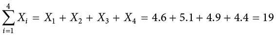
We label the weight of Grape 1 as , of Grape 2 as , etc. The following formula means to sum up the weights of the four grapes:

The Greek letter indicates summation. The “i = 1” at the bottom indicates that the summation is to start with , and the 4 at the top indicates that the summation will end with . The “” indicates that X is the variable to be summed as i goes from 1 to 4. Therefore,

The symbol

indicates that only the first 3 scores are to be summed. The index variable i goes from 1 to 3.

When all the scores of a variable (such as X) are to be summed, it is often convenient to use the following abbreviated notation:

Thus, when no values of i are shown, it means to sum all the values of X.

Many formulas involve squaring numbers before they are summed. This is indicated as

Notice that:

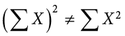
because the expression on the left means to sum up all the values of X and then square the sum (), whereas the expression on the right means to square the numbers and then sum the squares (90.54, as shown).

Some formulas involve the sum of cross products. Below are the data for variables X and Y. The cross products (XY) are shown in the third column. The sum of the cross products is .

X	Y	XY
1	3	3
2	2	4
3	7	21

In summation notation, this is written as:

Exercises

1. In your own words, describe why we study statistics.
2. For each of the following, determine if the variable is continuous or discrete:
   1. Time taken to read a book chapter
   2. Favorite food
   3. Cognitive ability
   4. Temperature
   5. Letter grade received in a class
3. For each of the following, determine the level of measurement:
   1. T-shirt size
   2. Time taken to run 100-meter race
   3. First, second, and third place in 100-meter race
   4. Birthplace
   5. Temperature in Celsius
4. What is the difference between a population and a sample? Which is described by a parameter and which is described by a statistic?
5. What is sampling bias? What is sampling error?
6. What is the difference between a simple random sample and a stratified random sample?
7. What are the two key characteristics of a true experimental design?
8. When would we use a quasi-experimental design?
9. Use the following dataset for the computations below:
   

   X	Y
   2	8
   3	8
   7	4
   5	1
   9	4

   1. 
   2. 
   3. 
   4. 
10. What are the most common measures of central tendency and spread?