6 Chapter 6: Sampling Distributions
We have come to the final chapter in this unit. We will now take the logic, ideas, and techniques we have developed and put them together to see how we can take a sample of data and use it to make inferences about what’s truly happening in the broader population. This is the final piece of the puzzle that we need to understand in order to have the groundwork necessary for formal hypothesis testing. Though some of the concepts in this chapter seem strange, they are all simple extensions of what we have already learned in previous chapters, especially Chapter 4 and Chapter 5.
People, Samples, and Populations
Most of what we have dealt with so far has concerned individual scores grouped into samples, with those samples being drawn from and, hopefully, representative of a population. We saw how we can understand the location of individual scores within a sample’s distribution via z scores, and how we can extend that to understand how likely it is to observe scores higher or lower than an individual score via probability.
Inherent in this work is the notion that an individual score will differ from the mean, which we quantify as a z score. All of the individual scores will differ from the mean in different amounts and different directions, which is natural and expected. We quantify these differences as variance and standard deviation. Measures of spread and the idea of variability in observations is a key principle in inferential statistics. We know that any observation, whether it is a single score, a set of scores, or a particular descriptive statistic will differ from the center of whatever distribution it belongs in.
This is equally true of things outside of statistics and format data collection and analysis. Some days you hear your alarm and wake up easily, but other days you need to hit snooze a few (dozen) times. Some days traffic is light, but other days it is very heavy. Some classes you are able to focus, pay attention, and take good notes, but other days you find yourself zoning out the entire time. Each individual observation is an insight but is not, by itself, the entire story, and it takes an extreme deviation from what we expect for us to think that something strange is going on. Being a little sleepy is normal, but being completely unable to get out of bed might indicate that we are sick. Light traffic is a good thing, but almost no cars on the road might make us think we forgot it is Saturday. Zoning out occasionally is fine, but if we cannot focus at all, we might be in a stats class rather than a fun one.
All of these principles carry forward from scores within samples to samples within populations. Just like an individual score will differ from its mean, an individual sample mean will differ from the true population mean. We encountered this principle in earlier chapters: sampling error. As mentioned way back in Chapter 1, sampling error is an incredibly important principle. We know ahead of time that if we collect data and compute a sample, the observed value of that sample will be at least slightly off from what we expect it to be based on our supposed population mean; this is natural and expected. However, if our sample mean is extremely different from what we expect based on the population mean, there may be something going on.
The Sampling Distribution of Sample Means
To see how we use sampling error, we will learn about a new, theoretical distribution known as the sampling distribution. In the same way that we can gather a lot of individual scores and put them together to form a distribution with a center and spread, if we were to take many samples, all of the same size, and calculate the mean of each of those, we could put those means together to form a distribution. This new distribution is, intuitively, known as the distribution of sample means. It is one example of what we call a sampling distribution, which can be formed from a set of any statistic, such as a mean, a test statistic, or a correlation coefficient (more on the latter two in Unit 2 and Unit 3). For our purposes, understanding the distribution of sample means will be enough to see how all other sampling distributions work to enable and inform our inferential analyses, so these two terms will be used interchangeably from here on out. Let’s take a deeper look at some of its characteristics.
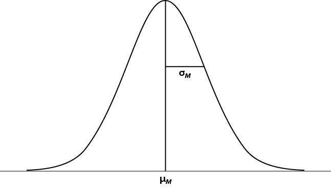
The sampling distribution of sample means can be described by its shape, center, and spread, just like any of the other distributions we have worked with. The shape of our sampling distribution is normal: a bell-shaped curve with a single peak and two tails extending symmetrically in either direction, just like what we saw in previous chapters. The center of the sampling distribution of sample means—which is, itself, the mean or average of the means—is the true population mean,  . This will sometimes be written as
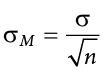
  to denote it as the mean of the sample means. The spread of the sampling distribution is called the standard error, the quantification of sampling error, denoted
  . The formula for standard error is:
Notice that the sample size is in this equation. As stated above, the sampling distribution refers to samples of a specific size. That is, all sample means must be calculated from samples of the same size n, such as n = 10, n = 30, or n = 100. This sample size refers to how many people or observations are in each individual sample, not how many samples are used to form the sampling distribution. This is because the sampling distribution is a theoretical distribution, not one we will ever actually calculate or observe. Figure 6.1 displays the principles stated here in graphical form.
Figure 6.1. The sampling distribution of sample means. (“Sampling Distribution of Sample Means” by Judy Schmitt is licensed under CC BY-NC-SA 4.0.)
Two Important Axioms
We just learned that the sampling distribution is theoretical: we never actually see it. If that is true, then how can we know it works? How can we use something we don’t see? The answer lies in two very important mathematical facts: the central limit theorem and the law of large numbers. We will not go into the math behind how these statements were derived, but knowing what they are and what they mean is important to understanding why inferential statistics work and how we can draw conclusions about a population based on information gained from a single sample.
Central Limit Theorem
The central limit theorem states:
For samples of a single size n, drawn from a population with a given mean and variance s2, the sampling distribution of sample means will have a mean  and variance
 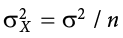 . This distribution will approach normality as n increases.
From this, we are able to find the standard deviation of our sampling distribution, the standard error. As you can see, just like any other standard deviation, the standard error is simply the square root of the variance of the distribution.
The last sentence of the central limit theorem states that the sampling distribution will be more normal as the sample size of the samples used to create it increases. What this means is that bigger samples will create a more normal distribution, so we are better able to use the techniques we developed for normal distributions and probabilities. So how large is large enough? In general, a sampling distribution will be normal if either of two characteristics is true: (1) the population from which the samples are drawn is normally distributed or (2) the sample size is equal to or greater than 30. This second criterion is very important because it enables us to use methods developed for normal distributions even if the true population distribution is skewed.
Law of Large Numbers
The law of large numbers simply states that as our sample size increases, the probability that our sample mean is an accurate representation of the true population mean also increases. It is the formal mathematical way to state that larger samples are more accurate.
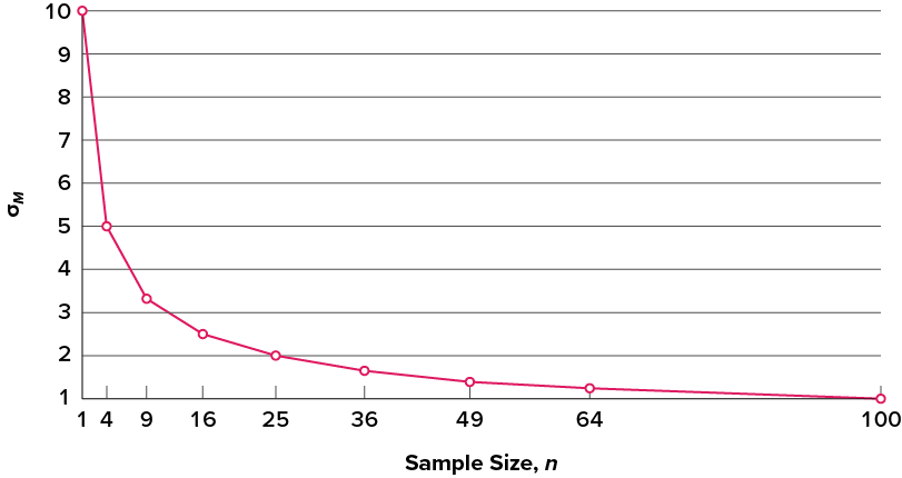
The law of large numbers is related to the central limit theorem, specifically the formulas for variance and standard error. Notice that the sample size appears in the denominators of those formulas. A larger denominator in any fraction means that the overall value of the fraction gets smaller (i.e., 1/2 = 0.50, 1/3 = 0.33, 1/4 = 0.25, and so on). Thus, larger sample sizes will create smaller standard errors. We already know that standard error is the spread of the sampling distribution and that a smaller spread creates a narrower distribution. Therefore, larger sample sizes create narrower sampling distributions, which increases the probability that a sample mean will be close to the center and decreases the probability that it will be in the tails. This is illustrated in Figure 6.2 and Figure 6.3.
Figure 6.2. Sampling distributions from the same population with m = 50 and s = 10 but different sample sizes (N = 10, N = 30, N = 50, N = 100). (“Sampling Distributions with Different Sample Sizes” by Judy Schmitt is licensed under CC BY-NC-SA 4.0.)
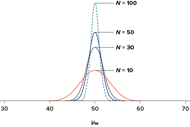
Figure 6.3. Relationship between sample size and standard error for a constant s = 10. (“Relationship between Sample Size and Standard Error” by Judy Schmitt is licensed under CC BY-NC-SA 4.0.)
Using Standard Error for Probability
In this chapter, we saw that we can use z scores to split up a normal distribution and calculate the proportion of the area under the curve in one of the new regions, giving us the probability of randomly selecting a z score in that range. We can follow the exact sample process for sample means, converting them into z scores and calculating probabilities. The only difference is that instead of dividing a raw score by the standard deviation, we divide the sample mean by the standard error.
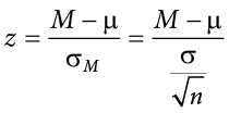
Let’s say we are drawing samples from a population with a mean of 50 and a standard deviation of 10 (the same values used in Figure 6.2). What is the probability that we get a random sample of size 10 with a mean greater than or equal to 55? That is, for n = 10, what is the probability that  ? First, we need to convert this sample mean score into a z score:

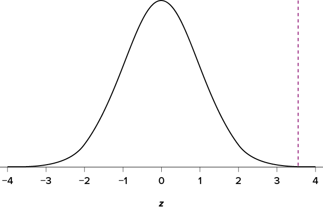
Now we need to shade the area under the normal curve corresponding to scores greater than z = 1.58, as in Figure 6.4.
Figure 6.4. Area under the curve greater than z = 1.58. (“Area under the Curve Greater than z1.58” by Judy Schmitt is licensed under CC BY-NC-SA 4.0.)
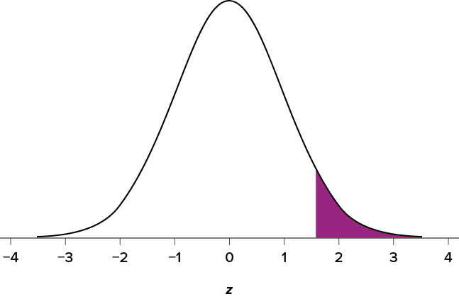
Now we go to our z table and find that the area to the left of z = 1.58 is .9429. Finally, because we need the area to the right (per our shaded diagram), we simply subtract this from 1 to get 1.00 − .9429 = .0571. So, the probability of randomly drawing a sample of 10 people from a population with a mean of 50 and standard deviation of 10 whose sample mean is 55 or more is p = .0571, or 5.71%. Notice that we are talking about means that are 55 or more. That is because, strictly speaking, it’s impossible to calculate the probability of a score taking on exactly 1 value since the “shaded region” would just be a line with no area to calculate.
Now let’s do the same thing, but assume that instead of only having a sample of 10 people we took a sample of 50 people. First, we find z:
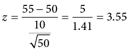
Then we shade the appropriate region of the normal distribution, as shown in Figure 6.5.
Figure 6.5. Area under the curve greater than z = 3.55. (“Area under the Curve Greater Than z3.55” by Judy Schmitt is licensed under CC BY-NC-SA 4.0.)
Notice that no region of Figure 6.5 appears to be shaded. That is because the area under the curve that far out into the tail is so small that it can’t even be seen (the red line has been added to show exactly where the region starts). Thus, we already know that the probability must be smaller for N = 50 than N = 10 because the size of the area (the proportion) is much smaller.
We run into a similar issue when we try to find z = 3.55 on our Standard Normal Distribution Table. The table only goes up to 3.09 because everything beyond that is almost 0 and changes so little that it’s not worth printing values. The closest we can get is subtracting the largest value, .9990, from 1 to get .001. We know that, technically, the actual probability is smaller than this (since 3.55 is farther into the tail than 3.09), so we say that the probability is p < .001, or less than 0.1%.
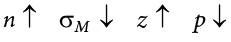
This example shows what an impact sample size can have. From the same population, looking for exactly the same thing, changing only the sample size took us from roughly a 5% chance (or about 1/20 odds) to a less than 0.1% chance (or less than 1 in 1000). As the sample size n increased, the standard error decreased, which in turn caused the value of z to increase, which finally caused the p value (a term for probability we will use a lot in Unit 2) to decrease. You can think of this relationship like gears: turning the first gear (sample size) clockwise causes the next gear (standard error) to turn counterclockwise, which causes the third gear (z) to turn clockwise, which finally causes the last gear (probability) to turn counterclockwise. All of these pieces fit together, and the relationships will always be the same:
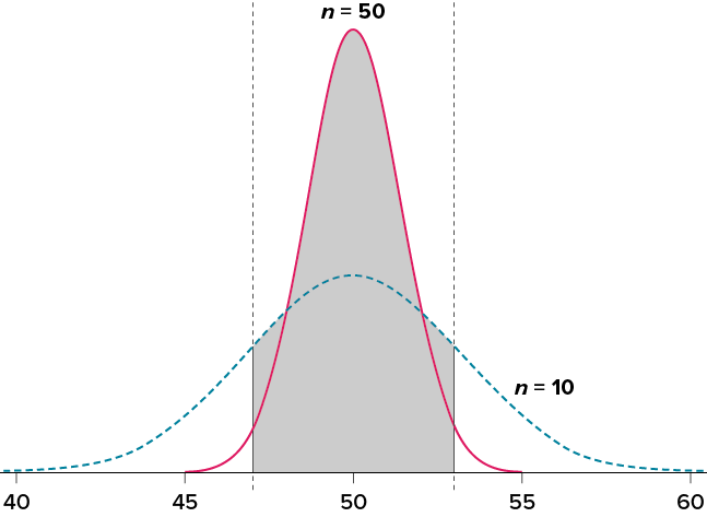
Let’s look at this one more way. For the same population of sample size 50 and standard deviation 10, what proportion of sample means fall between 47 and 53 if they are of sample size 10 and sample size 50?
We’ll start again with n = 10. Converting 47 and 53 into z scores, we get z = −0.95 and z = 0.95, respectively. From our z table, we find that the proportion between these two scores is .6578 (the process here is left off for the student to practice converting  to z and z to proportions). So, 65.78% of sample means of sample size 10 will fall between 47 and 53. For n = 50, our z scores for 47 and 53 are ±2.13, which gives us a proportion of the area as .9668, almost 97%! Shaded regions for each of these sampling distributions is displayed in Figure 6.6. The sampling distributions are shown on the original scale, rather than as z scores, so you can see the effect of the shading and how much of the body falls into the range, which is marked off with thin dotted lines.
Figure 6.6. Areas between 47 and 53 for sampling distributions of n = 10 and n = 50. (“Areas between 47 and 53” by Judy Schmitt is licensed under CC BY-NC-SA 4.0.)
Sampling Distribution, Probability, and Inference
We’ve seen how we can use the standard error to determine probability based on our normal curve. We can think of the standard error as how much we would naturally expect our statistic—be it a mean or some other statistic)—to vary. In our formula for z based on a sample mean, the numerator  is what we call an observed effect. That is, it is what we observe in our sample mean versus what we expected based on the population from which that sample mean was calculated.
Because the sample mean will naturally move around due to sampling error, our observed effect will also change naturally. In the context of our formula for z, then, our standard error is how much we would naturally expect the observed effect to change. Changing by a little is completely normal, but changing by a lot might indicate something is going on. This is the basis of inferential statistics and the logic behind hypothesis testing, the subject of Unit 2.
Exercises
- What is a sampling distribution?
- What are the two mathematical facts that describe how sampling distributions work?
- What is the difference between a sampling distribution and a regular distribution?
- What effect does sample size have on the shape of a sampling distribution?
- What is standard error?
- For a population with a mean of 75 and a standard deviation of 12, what proportion of sample means of size n = 16 fall above 82?
- For a population with a mean of 100 and standard deviation of 16, what is the probability that a random sample of size 4 will have a mean between 110 and 130?
- Find the z score for the following means taken from a population with mean 10 and standard deviation 2:
- M = 8, n = 12
- M = 8, n = 30
- M = 20, n = 4
- M = 20, n = 16
- As the sample size increases, what happens to the p value associated with a given sample mean?
- For a population with a mean of 35 and standard deviation of 7, find the sample mean of size n = 20 that cuts off the top 5% of the sampling distribution.
Answers to Odd-Numbered Exercises
1)
The sampling distribution (or sampling distribution of the sample means) is the distribution formed by combining many sample means taken from the same population and of a single, consistent sample size.
3)
A sampling distribution is made of statistics (e.g., the mean), whereas a regular distribution is made of individual scores.
5)
Standard error is the spread of the sampling distribution and is the quantification of sampling error. It is how much we expect the sample mean to naturally change based on random chance.
7)
10.46% or .1046
9)
As sample size increases, the p value will decrease.
