13 Chapter 13: Linear Regression

In Chapter 11, we learned about ANOVA, which involves a new way of looking at how our data are structured and the inferences we can draw from that. In Chapter 12, we learned about correlations, which analyze two continuous variables at the same time to see if they systematically relate in a linear fashion. In this chapter, we will combine these two techniques in an analysis called simple linear regression, or regression for short. Regression uses the technique of variance partitioning from ANOVA to more formally assess the types of relationships looked at in correlations. Regression is the most general and most flexible analysis covered in this book, and we will only scratch the surface.

Line of Best Fit

In correlations, we referred to a linear trend in the data. That is, we assumed that there was a straight line we could draw through the middle of our scatter plot that would represent the relationship between our two variables, X and Y. Regression involves solving for the equation of that line, which is called the line of best fit.

The line of best fit can be thought of as the central tendency of our scatter plot. The term best fit means that the line is as close to all points (with each point representing both variables for a single person) in the scatter plot as possible, with a balance of scores above and below the line. This is the same idea as the mean, which has an equal weighting of scores above and below it and is the best singular descriptor of all our data points for a single variable.

We have already seen many scatter plots in Chapter 2 and Chapter 12, so we know by now that no scatter plot has points that form a perfectly straight line. Because of this, when we put a straight line through a scatter plot, it will not touch all of the points, and it may not even touch any! This will result in some distance between the line and each of the points it is supposed to represent, just like a mean has some distance between it and all of the individual scores in the dataset.

The distances between the line of best fit and each individual data point go by two different names that mean the same thing: errors and residuals. The term error in regression is closely aligned with the meaning of error in statistics (think standard error or sampling error); it does not mean that we did anything wrong, it simply means that there was some discrepancy or difference between what our analysis produced and the true value we are trying to get at. The term residual is new to our study of statistics, and it takes on a very similar meaning in regression to what it means in everyday parlance: there is something left over. In regression, what is “left over”—that is, what makes up the residual—is an imperfection in our ability to predict values of the Y variable using our line. This definition brings us to one of the primary purposes of regression and the line of best fit: predicting scores.

Prediction

The goal of regression is the same as the goal of ANOVA: to take what we know about one variable (X) and use it to explain our observed differences in another variable (Y). In ANOVA, we talked about—and tested for—group mean differences, but in regression we do not have groups for our explanatory variable; we have a continuous variable, like in correlation. Because of this, our vocabulary will be a little bit different, but the process, logic, and end result are all the same.

In regression, we most frequently talk about prediction, specifically predicting our outcome variable Y from our explanatory variable X, and we use the line of best fit to make our predictions. Let’s take a look at the equation for the line, which is quite simple:

Ŷ = a + bX

The terms in the equation are defined as:

Ŷ: the predicted value of Y for an individual person

a: the intercept of the line

b: the slope of the line

X: the observed value of X for an individual person

What this shows us is that we will use our known value of X for each person to predict the value of Y for that person. The predicted value, Ŷ (“Y-hat”), is our best guess for what a person’s score on the outcome is. Notice also that the form of the equation is very similar to very simple linear equations that you have likely encountered before and has only two parameter estimates: an intercept (where the line crosses the y-axis) and a slope (how steep—and the direction, positive or negative—the line is). These are parameter estimates because, like everything else in statistics, we are interested in approximating the true value of the relationship in the population but can only ever estimate it using sample data. We will soon see that one of these parameters, the slope, is the focus of our hypothesis tests (the intercept is only there to make the math work out properly and is rarely interpretable). The formulas for these parameter estimates use very familiar values:

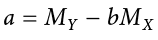
We have seen each of these before. and are the means of Y and X, respectively; is the covariance of X and Y we learned about with correlations; and is the variance of X. The formula for the slope is very similar to the formula for a Pearson correlation coefficient; the only difference is that we are dividing by the variance of X instead of the product of the standard deviations of X and Y. Because of this, our slope is scaled to the same scale as our X variable and is no longer constrained to be between 0 and 1 in absolute value. This formula provides a clear definition of the slope of the line of best fit, and just like with correlation, this definitional formula can be simplified into a short computational formula for easier calculations. In this case, we are simply taking the sum of products and dividing by the sum of squares for X.

Notice that there is a third formula for the slope of the line that involves the correlation between X and Y. This is because regression and correlation look for the same thing: a straight line through the middle of the data. The only difference between a regression coefficient in simple linear regression and a Pearson correlation coefficient is the scale. So, if you lack raw data but have summary information on the correlation and standard deviations for variables, you can still compute a slope, and therefore an intercept, for a line of best fit.

It is important to point out that the Y values in the equations for a and b are our observed Y values in the dataset, not the predicted Y values (Ŷ) from our equation for the line of best fit. Thus, we will have three values for each person: the observed value of X (X), the observed value of Y (Y), and the predicted value of Y (Ŷ). You may be asking why we would try to predict Y if we have an observed value of Y, and that is a reasonable question. The answer has two explanations. First, we need to use known values of Y to calculate the parameter estimates in our equation, and we use the difference between our observed values and predicted values (Y − Ŷ) to see how accurate our equation is. And second, we often use regression to create a predictive model that we can then use to predict values of Y for other people for whom we only have information on X.

Let’s look at this from an applied example. Businesses often have more applicants for a job than they have openings available, so they want to know who among the applicants is most likely to be the best employee. There are many criteria that can be used, but one is a personality test for conscientiousness, with the belief being that more conscientious (more responsible) employees are better than less conscientious employees. A business might give their employees a personality inventory to assess conscientiousness and study existing performance data to look for a relationship. In this example, we have known values of the predictor (X, conscientiousness) and outcome (Y, job performance), so we can estimate an equation for a line of best fit and see how accurately conscientiousness predicts job performance, then use this equation to predict future job performance of applicants based only on their known values of conscientiousness from personality inventories given during the application process.

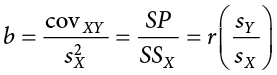
The key in assessing whether a linear regression works well is the difference between our observed and known Y values and our predicted Ŷ values. As mentioned in passing above, we use subtraction to find the difference between them (Y − Ŷ) in the same way we use subtraction for deviation scores and sums of squares. The value (Y − Ŷ) is our residual, which, as defined above, is how close our line of best fit is to our actual values. We can visualize residuals to get a better sense of what they are by creating a scatter plot and overlaying a line of best fit on it, as shown in Figure 13.1.

In Figure 13.1, the triangular dots represent observations from each person on both X and Y and the dotted line is the line of best fit estimated by the equation Ŷ = a + bX. For every person in the dataset, the line represents their predicted score. The brackets between the triangular dots and the predicted scores on the line of best fit are our residuals. (For ease of viewing, they are only drawn for four observations, but in reality there is one for every observation.) You can see that some residuals are positive and some are negative, and that some are very large and some are very small. This means that some predictions are very accurate and some are very inaccurate, and that some predictions overestimate values and some underestimate values. Across the entire dataset, the line of best fit is the one that minimizes the total (sum) value of all residuals. That is, although predictions at an individual level might be somewhat inaccurate, across our full sample and (theoretically) in future samples our total amount of error is as small as possible. We call this property of the line of best fit the least squares error solution. This term means that the solution—or equation—of the line is the one that provides the smallest possible value of the squared errors (squared so that they can be summed, just like in standard deviation) relative to any other straight line we could draw through the data.

Predicting Scores and Explaining Variance

We have now seen that the purpose of regression is twofold: we want to predict scores based on our line and, as stated earlier, explain variance in our observed Y variable just like in ANOVA. These two purposes go hand in hand, and our ability to predict scores is literally our ability to explain variance. That is, if we cannot account for the variance in Y based on X, then we have no reason to use X to predict future values of Y.

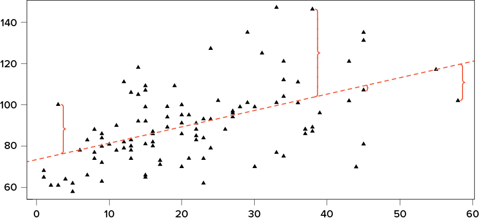
We know that the overall variance in Y is a function of each score deviating from the mean of Y (as in our calculation of variance and standard deviation). So, just like the brackets in Figure 13.1 representing residuals, given as (Y − Ŷ), we can visualize the overall variance as each score’s distance from the overall mean of Y, given as (), our normal deviation score. This is shown in Figure 13.2.

In Figure 13.2, the solid line is the mean of Y, and the blue brackets are the deviation scores between our observed values of Y and the mean of Y. This represents the overall variance that we are trying to explain. Thus, the residuals and the deviation scores are the same type of idea: the distance between an observed score and a given line, either the line of best fit that gives predictions or the line representing the mean that serves as a baseline. The difference between these two values, which is the distance between the lines themselves, is our model’s ability to predict scores above and beyond the baseline mean; that is, it is our model’s ability to explain the variance we observe in Y based on values of X. If we have no ability to explain variance, then our line will be flat (the slope will be 0.00) and will be the same as the line representing the mean, and the distance between the lines will be 0.00 as well.

We now have three pieces of information: the distance from the observed score to the mean, the distance from the observed score to the prediction line, and the distance from the prediction line to the mean. These are our three pieces of information needed to test our hypotheses about regression and to calculate effect sizes. They are our three sums of squares, just like in ANOVA. Our distance from the observed score to the mean is the sum of squares total, which we are trying to explain. Our distance from the observed score to the prediction line is our sum of squares error, or residual, which we are trying to minimize. Our distance from the prediction line to the mean is our sum of squares model, which is our observed effect and our ability to explain variance. Each of these will go into the ANOVA table to calculate our test statistic.

ANOVA Table

Our ANOVA table in regression follows the exact same format as it did for ANOVA (hence the name). The top row (Model) is our observed effect, the middle row is our error, and the bottom row is our total. The columns take on the same interpretations as well: from left to right, we have our sums of squares, our degrees of freedom, our mean squares, and our F statistic.

As with ANOVA, getting the values for the SS column is a straightforward but somewhat arduous process. First, you take the raw scores of X and Y and calculate the means, variances, and covariance using the sum of products table introduced in our chapter on correlations. Next, you use the variance of X and the covariance of X and Y to calculate the slope of the line, b. (The formula for calculating b was provided earlier.) After that, you use the means and the slope to find the intercept, a, which is given alongside b. After that, you use the full prediction equation for the line of best fit to get predicted Y scores (Ŷ) for each person. Finally, you use the observed Y scores, predicted Y scores, and mean of Y () to find the appropriate deviation scores for each person for each sum of squares source in the table and sum them to get the sum of squares model, sum of squares error, and sum of squares total. As with ANOVA, you won’t be required to compute the SS values by hand, but you will need to know what they represent and how they fit together.

The other columns in the ANOVA table are all familiar. The degrees of freedom column still has N − 1 for our total, but now we have N − 2 for our error degrees of freedom and 1 for our model degrees of freedom; this is because simple linear regression only has one predictor, so our degrees of freedom for the model is always 1 and does not change. The total degrees of freedom must still be the sum of the other two, so our degrees of freedom error will always be N − 2 for simple linear regression. The mean square columns are still the SS column divided by the df column, and the test statistic F is still the ratio of the mean squares. Based on this, it is now explicitly clear that not only do regression and ANOVA have the same goal but they are, in fact, the same analysis entirely. The only difference is the type of data we feed into the predictor side of the equations: continuous for regression and categorical for ANOVA.

Hypothesis Testing in Regression

Regression, like all other analyses, will test a null hypothesis in our data. In regression, we are interested in predicting Y scores and explaining variance using a line, the slope of which is what allows us to get closer to our observed scores than the mean of Y can. Thus, our hypotheses concern the slope of the line, which is estimated in the prediction equation by b (the slope of a population, as opposed to b, which is the slope of a sample). Specifically, we want to test that the slope is not zero:

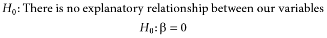
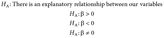
A non-zero slope indicates that we can explain values in Y based on X and therefore predict future values of Y based on X. Our alternative hypotheses are analogous to those in correlation: positive relationships have values above zero, negative relationships have values below zero, and two-tailed tests are possible. Just like ANOVA, we will test the significance of this relationship using the F statistic calculated in our ANOVA table compared to a critical value from the F distribution table. Let’s take a look at an example and regression in action.

Example Happiness and Well-being

Researchers are interested in explaining differences in how happy people are based on how healthy people are. They gather data on each of these variables from 18 people and fit a linear regression model to explain the variance. We will follow the four-step hypothesis-testing procedure to see if there is a relationship between these variables that is statistically significant.

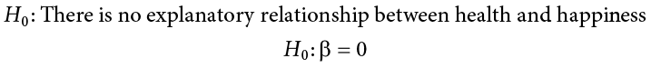
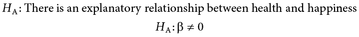
Step 1: State the Hypotheses

The null hypothesis in regression states that there is no relationship between our variables. The alternative states that there is a relationship, but because our research description did not explicitly state a direction of the relationship, we will use a non-directional hypothesis.

Step 2: Find the Critical Value

Because regression and ANOVA are the same analysis, our critical value for regression will come from the same place: the F distribution table, which uses two types of degrees of freedom. We saw in the ANOVA table that the degrees of freedom for our numerator—the Model line—is always 1 in simple linear regression, and that the denominator degrees of freedom—from the Error line—is N − 2. In this instance, we have 18 people so our degrees of freedom for the denominator is 16. Going to our F table (a portion of which is shown in Table 13.1), we find that the appropriate critical value for 1 and 16 degrees of freedom is F* = 4.49. (The complete F table can be found in Appendix C.)

Step 3: Calculate the Test Statistic and Effect Size

The process of calculating the test statistic for regression first involves computing the parameter estimates for the line of best fit. To do this, we first calculate the means, standard deviations, and sum of products for our X and Y variables, as shown below.

From the raw data in our X and Y columns, we find that the means are = 19.78 and = 17.45. The deviation scores for each variable sum to zero, so all is well there. The sums of squares for X and Y ultimately lead us to standard deviations of sX = 2.12 and sY = 3.20. Finally, our sum of products is 58.29, which gives us a covariance of covXY = 3.43, so we know our relationship will be positive. This is all the information we need for our equations for the line of best fit.

First, we must calculate the slope of the line:

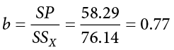
This means that as X changes by 1 unit, Y will change by 0.77. In terms of our problem, as health increases by 1, happiness goes up by 0.77, which is a positive relationship. Next, we use the slope, along with the means of each variable, to compute the intercept:

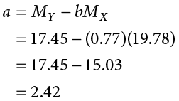
For this particular problem (and most regressions), the intercept is not an important or interpretable value, so we will not read into it further. Now that we have all of our parameters estimated, we can give the full equation for our line of best fit:

Ŷ = 2.42 + 0.77X

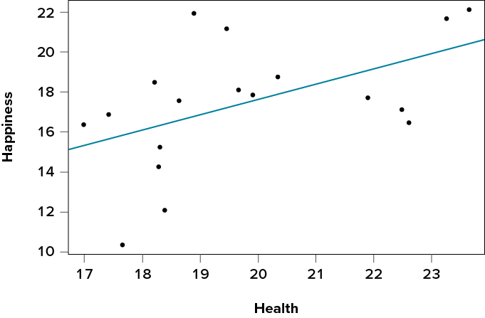
We can plot this relationship in a scatter plot and overlay our line onto it, as shown in Figure 13.3.

We can use the line equation to find predicted values for each observation and use them to calculate our sums of squares model and error, but this is tedious to do by hand, so we will let the computer software do the heavy lifting in that column of our ANOVA table:

Now that we have these, we can fill in the rest of the ANOVA table. We already found our degrees of freedom in Step 2:

Our total line is always the sum of the other two lines, giving us:

Our mean squares column is only calculated for the model and error lines and is always our SS divided by our df, which is:

Finally, our F statistic is the ratio of the mean squares:

This gives us an obtained F statistic of 5.52, which we will use to test our hypothesis.

Effect Size in Regression

We know that, because our statistic is significant, we should calculate an effect size. In regression, our effect size is variance explained, just like it was in ANOVA. Instead of using h2 to represent this, we instead use R2, as we saw in correlation—yet more evidence that all of these are the same analysis. (Note that in regression analysis, R2 is typically capitalized, although for simple linear regression it represents the same value as r2 we used in correlation.) Variance explained is still the ratio of SSM to SST:

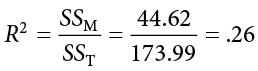
We are explaining 26% of the variance in happiness based on health, which is a large effect size. (R2 uses the same effect size cutoffs as h2.)

Step 4: Make the Decision

We now have everything we need to make our final decision. Our obtained test statistic was F = 5.52 and our critical value was F* = 4.49. Since our obtained test statistic is greater than our critical value, we can reject the null hypothesis.

Reject H0. Based on our sample of 18 people, we can predict levels of happiness based on how healthy someone is, and the effect size was large, F(1, 16) = 5.52, p < .05, R2 < .26.

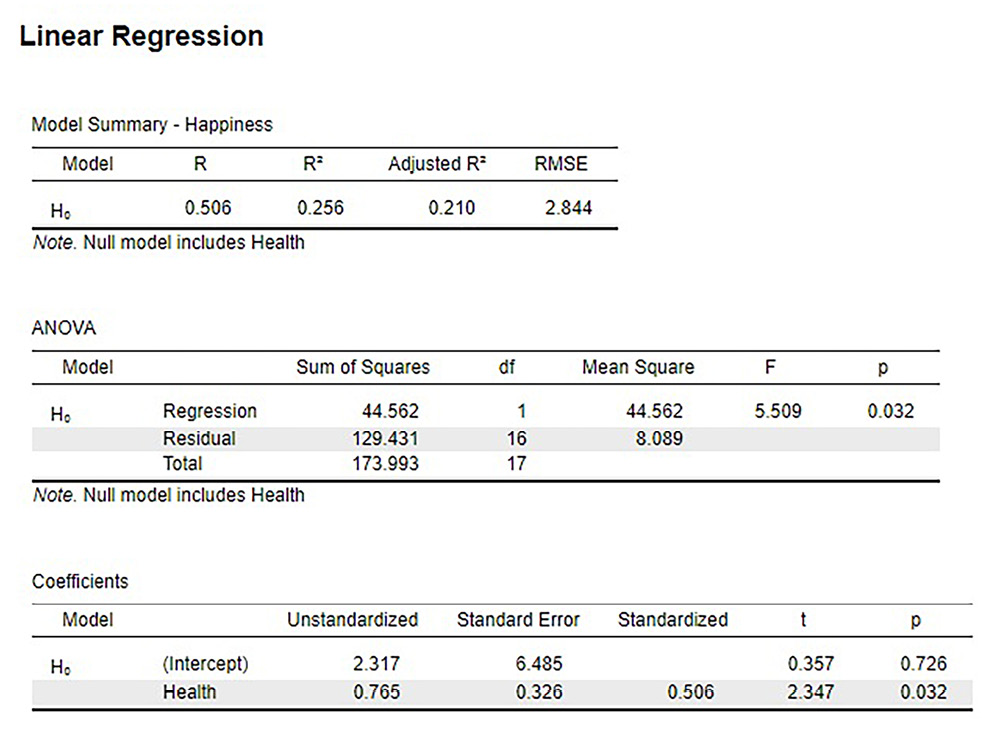
Figure 13.4 shows the output from JASP for this example.

Accuracy in Prediction

We found a large, statistically significant relationship between our variables, which is what we hoped for. However, if we want to use our estimated line of best fit for future prediction, we will also want to know how precise or accurate our predicted values are. What we want to know is the average distance from our predictions to our actual observed values, or the average size of the residual (Y − Ŷ). The average size of the residual is known by a specific name: the standard error of the estimate (), which is given by the formula

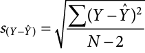
This formula is almost identical to our standard deviation formula, and it follows the same logic. We square our residuals, add them up, then divide by the degrees of freedom. Although this sounds like a long process, we already have the sum of the squared residuals in our ANOVA table! In fact, the value under the square root sign is just the SSE divided by the dfE, which is called the mean squared error, or MSE:

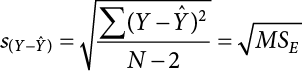
For our example:

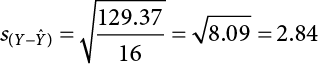
So on average, our predictions are just under 3 points away from our actual values. There are no specific cutoffs or guidelines for how big our standard error of the estimate can or should be; it is highly dependent on both our sample size and the scale of our original Y variable, so expert judgment should be used. In this case, the estimate is not that far off and can be considered reasonably precise.

Multiple Regression and Other Extensions

Simple linear regression as presented here is only a stepping stone toward an entire field of research and application. Regression is an incredibly flexible and powerful tool, and the extensions and variations on it are far beyond the scope of this chapter. (Indeed, even entire books struggle to accommodate all possible applications of the simple principles laid out here.) The next step in regression is to study multiple regression, which uses multiple X variables as predictors for a single Y variable at the same time. The math of multiple regression is very complex but the logic is the same: we are trying to use variables that are statistically significantly related to our outcome to explain the variance we observe in that outcome. Other forms of regression include curvilinear models that can explain curves in the data rather than the straight lines used here, as well as moderation models that change the relationship between two variables based on levels of a third. The possibilities are truly endless and offer a lifetime of discovery.

Exercises

1. How are ANOVA and linear regression similar? How are they different?
2. What is a residual?
3. How are correlation and regression similar? How are they different?
4. What are the two parameters of the line of best fit, and what do they represent?
5. What is our criterion for finding the line of best fit?
6. Fill out the rest of the ANOVA tables below for simple linear regressions:

   1. Source	SS	df	MS	F
      Model	34.21
      Error
      Total	66.12	54

   2. Source	SS	df	MS	F
      Model			6.03
      Error		16
      Total	19.98

7. In Chapter 12, we found a statistically significant correlation between overall performance in class and how much time someone studied. Use the summary statistics calculated in that problem ( = 1.61, sX = 1.12, = 2.95, sY = 0.99, r = .65) to compute a line of best fit predicting success from study times.
8. Using the line of best fit equation created in Problem 7, predict the scores for how successful people will be based on how much they study:
   1. X = 1.20
   2. X = 3.33
   3. X = 0.71
   4. X = 4.00
9. You have become suspicious that the draft rankings of your fantasy football league have no predictive value for how teams place at the end of the season. You go back to historical league data and find rankings of teams after the draft and at the end of the season (shown in the following table) to test for a statistically significant predictive relationship. Assume SSM = 2.65 and SSE = 337.35.
   

   Draft Projection	Final Rankings
   1	14
   2	6
   3	8
   4	13
   5	2
   6	15
   7	4
   8	10
   9	11
   10	16
   11	9
   12	7
   13	14
   14	12
   15	1
   16	5

10. You have summary data for two variables: how extroverted someone is (X) and how often someone volunteers (Y). Using these values, calculate the line of best fit predicting volunteering from extroversion, then test for a statistically significant relationship using the hypothesis-testing procedure: = 12.58, sX = 4.65, = 7.44, sY = 2.12, r = .34, N = 67, SSM = 19.79, SSE = 215.77.