3 Chapter 3: Measures of Central Tendency and Spread
Now that we have visualized our data to understand its shape, we can begin with numerical analyses. The descriptive statistics presented in this chapter serve to describe the distribution of our data objectively and mathematically—our first step into statistical analysis! The topics here will serve as the basis for everything we do in the rest of the course.
What Is Central Tendency?
What is central tendency, and why do we want to know the central tendency of a group of scores? Let us first try to answer these questions intuitively. Then we will proceed to a more formal discussion.
Imagine this situation: You are in a class with just four other students, and the five of you took a 5-point pop quiz. Today your instructor is walking around the room, handing back the quizzes. She stops at your desk and hands you your paper. Written in bold black ink on the front is “3/5.” How do you react? Are you happy with your score of 3 or disappointed? How do you decide? You might calculate your percentage correct, realize it is 60%, and be appalled. But it is more likely that when deciding how to react to your performance, you will want additional information. What additional information would you like?
If you are like most students, you will immediately ask your classmates, “What’d ya get?” and then ask the instructor, “How did the class do?” In other words, the additional information you want is how your quiz score compares to other students’ scores. You therefore understand the importance of comparing your score to the class distribution of scores. Should your score of 3 turn out to be among the higher scores, then you’ll be pleased after all. On the other hand, if 3 is among the lower scores in the class, you won’t be quite so happy.
This idea of comparing individual scores to a distribution of scores is fundamental to statistics. So let’s explore it further, using the same example (the pop quiz you took with your four classmates). Three possible outcomes are shown in Table 3.1. They are labeled “Dataset A,” “Dataset B,” and “Dataset C.” Which of the three datasets would make you happiest? In other words, in comparing your score with your fellow students’ scores, in which dataset would your score of 3 be the most impressive?
In Dataset A, everyone’s score is 3. This puts your score at the exact center of the distribution. You can draw satisfaction from the fact that you did as well as everyone else. But of course it cuts both ways: everyone else did just as well as you.
Now consider the possibility that the scores are described as in Dataset B. This is a depressing outcome even though your score is no different than the one in Dataset A. The problem is that the other four students had higher grades, putting yours below the center of the distribution.
Finally, let’s look at Dataset C. This is more like it! All of your classmates score lower than you, so your score is above the center of the distribution.
Now let’s change the example in order to develop more insight into the center of a distribution. Figure 3.1 shows the results of an experiment on memory for chess positions. Subjects were shown a chess position and then asked to reconstruct it on an empty chess board. The number of pieces correctly placed was recorded. This was repeated for two more chess positions. The scores represent the total number of chess pieces correctly placed for the three chess positions. The maximum possible score was 89.
Figure 3.1. Back-to-back stem-and-leaf display. The left side shows the memory scores of the non-players. The right side shows the scores of the tournament players. (“Memory Scores Back-to-Back Stem and Leaf” by Judy Schmitt is licensed under CC BY-NC-SA 4.0.)
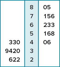
Two groups are compared. On the left are people who don’t play chess. On the right are people who play a great deal (tournament players). It is clear that the location of the center of the distribution for the non-players is much lower than the center of the distribution for the tournament players.
We’re sure you get the idea now about the center of a distribution. It is time to move beyond intuition. We need a formal definition of the center of a distribution. In fact, we’ll offer you three definitions! This is not just generosity on our part. There turn out to be (at least) three different ways of thinking about the center of a distribution, all of them useful in various contexts. In the remainder of this section we attempt to communicate the idea behind each concept. In the succeeding sections we will give statistical measures for these concepts of central tendency.
Definitions of Center
Now we explain the three measures of central tendency: (1) the point on which a distribution will balance, (2) the value whose average absolute deviation from all the other values is minimized, and (3) the value whose squared deviation from all the other values is minimized.
Balance Scale
One definition of central tendency is the point at which the distribution is in balance. Figure 3.2 shows the distribution of the five numbers 2, 3, 4, 9, 16 placed upon a balance scale. If each number weighs one pound, and is placed at its position along the number line, then it would be possible to balance them by placing a fulcrum at a particular point.
Figure 3.2. A balance scale. (“Balance Scale” by Judy Schmitt is licensed under CC BY-NC-SA 4.0.)

For another example, consider the distribution shown in Figure 3.3. It is balanced by placing the fulcrum in the geometric middle.
Figure 3.3. A distribution balanced on the tip of a triangle. (“Balanced Distribution” by Judy Schmitt is licensed under CC BY-NC-SA 4.0.)
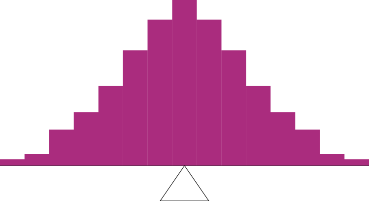
Figure 3.4 illustrates that the same distribution can’t be balanced by placing the fulcrum to the left of center.
Figure 3.4. The distribution is not balanced. (“Unbalanced Distribution” by Judy Schmitt is licensed under CC BY-NC-SA 4.0.)
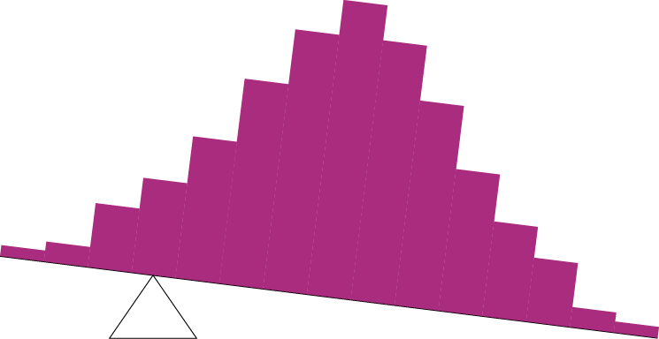
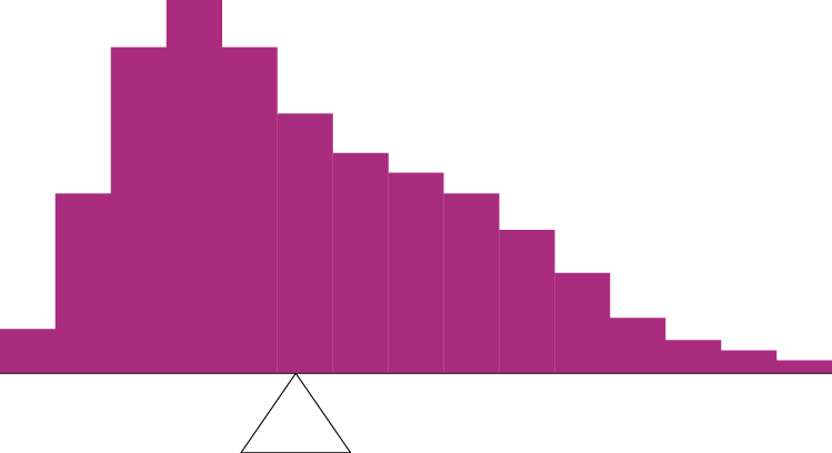
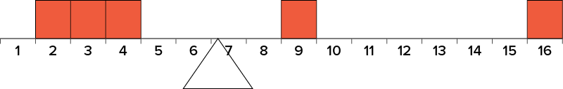
Figure 3.5 shows an asymmetric distribution. To balance it, we cannot put the fulcrum halfway between the lowest and highest values (as we did in Figure 3.3). Placing the fulcrum at the “half way” point would cause it to tip towards the left.
Figure 3.5. An asymmetric distribution balanced on the tip of a triangle. (“Asymmetric Distribution” by Judy Schmitt is licensed under CC BY-NC-SA 4.0.)
Smallest Absolute Deviation
Another way to define the center of a distribution is based on the concept of the sum of the absolute deviations (differences). Consider the distribution made up of the five numbers 2, 3, 4, 9, 16. Let’s see how far the distribution is from 10 (picking a number arbitrarily). Table 3.2 shows the sum of the absolute deviations of these numbers from the number 10.
The first row of the table shows that the absolute value of the difference between 2 and 10 is 8; the second row shows that the absolute difference between 3 and 10 is 7, and similarly for the other rows. When we add up the five absolute deviations, we get 28. So, the sum of the absolute deviations from 10 is 28. Likewise, the sum of the absolute deviations from 5 equals 3 + 2 + 1 + 4 + 11 = 21. So, the sum of the absolute deviations from 5 is smaller than the sum of the absolute deviations from 10. In this sense, 5 is closer, overall, to the other numbers than is 10.
We are now in a position to define a second measure of central tendency, this time in terms of absolute deviations. Specifically, according to our second definition, the center of a distribution is the number for which the sum of the absolute deviations is smallest. As we just saw, the sum of the absolute deviations from 10 is 28 and the sum of the absolute deviations from 5 is 21. Is there a value for which the sum of the absolute deviations is even smaller than 21? Yes. For these data, there is a value for which the sum of absolute deviations is only 20. See if you can find it.
Smallest Squared Deviation
We shall discuss one more way to define the center of a distribution. It is based on the concept of the sum of squared deviations (differences). Again, consider the distribution of the five numbers 2, 3, 4, 9, 16. Table 3.3 shows the sum of the squared deviations of these numbers from the number 10.
The first row in the table shows that the squared value of the difference between 2 and 10 is 64; the second row shows that the squared difference between 3 and 10 is 49, and so forth. When we add up all these squared deviations, we get 186.
Changing the target from 10 to 5, we calculate the sum of the squared deviations from 5 as 9 + 4 + 1 + 16 + 121 = 151. So, the sum of the squared deviations from 5 is smaller than the sum of the squared deviations from 10. Is there a value for which the sum of the squared deviations is even smaller than 151? Yes, it is possible to reach 134.8. Can you find the target number for which the sum of squared deviations is 134.8?
The target that minimizes the sum of squared deviations provides another useful definition of central tendency (the last one to be discussed in this section). It can be challenging to find the value that minimizes this sum.
Measures of Central Tendency
In the previous section we saw that there are several ways to define central tendency. This section defines the three most common measures of central tendency: the mean, the median, and the mode. The relationships among these measures of central tendency and the definitions given in the previous section will probably not be obvious to you.
This section gives only the basic definitions of the mean, median and mode. A further discussion of the relative merits and proper applications of these statistics is presented in a later section.
Arithmetic Mean
The arithmetic mean—the sum of the numbers divided by the number of numbers—is the most common measure of central tendency. The symbol “ ” (pronounced “mew”) is used for the mean of a population. The symbol
  is used for the mean of a sample. (In advanced statistics textbooks, the symbol
  , pronounced “x bar,” may be used to represent the mean of a sample.) The formula for is shown below:
where  is the sum of all the numbers in the population and
  is the number of numbers in the population.
The formula for is essentially identical:
where is the sum of all the numbers in the sample and n is the number of numbers in the sample. The only distinction between these two equations is whether we are referring to the population (in which case we use and ) or a sample of that population (in which case we use and n).
As an example, the mean of the numbers 1, 2, 3, 6, 8 is 20/5 = 4 regardless of whether the numbers constitute the entire population or just a sample from the population.
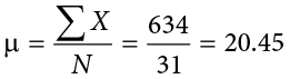
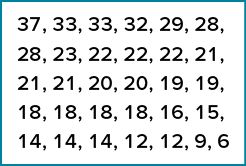
Figure 3.6 shows the number of touchdown (TD) passes thrown by each of the 31 teams in the National Football League in the 2000 season. The mean number of touchdown passes thrown is 20.45, as shown below.
Although the arithmetic mean is not the only “mean” (there is also a geometric mean, a harmonic mean, and many others that are all beyond the scope of this course), it is by far the most commonly used. Therefore, if the term “mean” is used without specifying whether it is the arithmetic mean, the geometric mean, or some other mean, it is assumed to refer to the arithmetic mean.
Figure 3.6. Number of touchdown passes. (“Touchdown Passes Raw Data” by Judy Schmitt is licensed under CC BY-NC-SA 4.0.)
Median
The median is also a frequently used measure of central tendency. The median is the midpoint of a distribution: the same number of scores is above the median as below it. For the data in Figure 3.6, there are 31 scores. The 16th highest score (which equals 20) is the median because there are 15 scores below the 16th score and 15 scores above the 16th score. The median can also be thought of as the 50th percentile.
When there is an odd number of numbers, the median is simply the middle number. For example, the median of 2, 4, and 7 is 4. When there is an even number of numbers, the median is the mean of the two middle numbers. Thus, the median of the numbers 2, 4, 7, 12 is:
When there are numbers with the same values, each appearance of that value gets counted. For example, in the set of numbers 1, 3, 4, 4, 5, 8, and 9, the median is 4 because there are three numbers (1, 3, and 4) below it and three numbers (5, 8, and 9) above it. If we only counted 4 once, the median would incorrectly be calculated at 4.5 (4 + 5, divided by 2). When in doubt, writing out all of the numbers in order and marking them off one at a time from the top and bottom will always lead you to the correct answer.
Mode
The mode is the most frequently occurring value in the dataset. For the data in Figure 3.6, the mode is 18 since more teams (4) had 18 touchdown passes than any other number of touchdown passes. With continuous data, such as response time measured to many decimals, the frequency of each value is one since no two scores will be exactly the same (see discussion of continuous variables). Therefore the mode of continuous data is normally computed from a grouped frequency distribution. Table 3.4 shows a grouped frequency distribution for the target response time data. Since the interval with the highest frequency is 600 to 700, the mode is the middle of that interval (650). Although the mode is not frequently used for continuous data, it is nevertheless an important measure of central tendency as it is the only measure we can use on qualitative or categorical data.
More on the Mean and Median
In the section What Is Central Tendency?, we saw that the center of a distribution could be defined three ways: (1) the point on which a distribution would balance, (2) the value whose average absolute deviation from all the other values is minimized, and (3) the value whose squared deviation from all the other values is minimized. The mean is the point on which a distribution would balance, the median is the value that minimizes the sum of absolute deviations, and the mean is the value that minimizes the sum of the squared deviations.
Table 3.5 shows the absolute and squared deviations of the numbers 2, 3, 4, 9, and 16 from their median of 4 and their mean of 6.8. You can see that the sum of absolute deviations from the median (20) is smaller than the sum of absolute deviations from the mean (22.8). On the other hand, the sum of squared deviations from the median (174) is larger than the sum of squared deviations from the mean (134.8).
Table 3.5. Absolute and squared deviations from the median of 4 and the mean of 6.8.
|
Value |
Absolute Deviation from Median |
Absolute Deviation from Mean |
Squared Deviation from Median |
Squared Deviation from Mean |
|
2 |
2 |
4.8 |
4 |
23.04 |
|
3 |
1 |
3.8 |
1 |
14.44 |
|
4 |
0 |
2.8 |
0 |
7.84 |
|
9 |
5 |
2.2 |
25 |
4.84 |
|
16 |
12 |
9.2 |
144 |
84.64 |
|
Total |
20 |
22.8 |
174 |
134.80 |
Figure 3.7 shows that the distribution balances at the mean of 6.8 and not at the median of 4. The relative advantages and disadvantages of the mean and median are discussed in the section Comparing Measures of Central Tendency.
Figure 3.7. The distribution balances at the mean of 6.8 and not at the median of 4.0. (“Balance Scale Numbered” by Judy Schmitt is licensed under CC BY-NC-SA 4.0.)
When a distribution is symmetric, then the mean and the median are the same. Consider the following distribution: 1, 3, 4, 5, 6, 7, 9. The mean and median are both 5. The mean, median, and mode are identical in the bell-shaped normal distribution.
Comparing Measures of Central Tendency
How do the various measures of central tendency compare with each other? For symmetric distributions, the mean and median are the same value, as is the mode except in bimodal distributions. However, differences among the measures occur with skewed distributions. Figure 3.8 shows the distribution of 642 scores on an introductory psychology test. Notice this distribution has a slight positive skew.
Figure 3.8. A distribution with a positive skew. (“Psychology Test Scores Histogram” by Judy Schmitt is licensed under CC BY-NC-SA 4.0.)
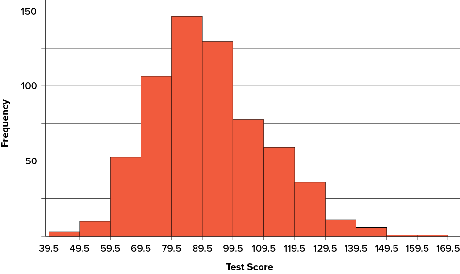
Measures of central tendency are shown in Table 3.6. Notice they do not differ greatly, with the exception that the mode is considerably lower than the other measures. When distributions have a positive skew, the mean is typically higher than the median, although it may not be in bimodal distributions. For these data, the mean of 91.58 is higher than the median of 90. This pattern holds true for any skew: the mode will remain at the highest point in the distribution, the median will be pulled slightly out into the skewed tail (the longer end of the distribution), and the mean will be pulled the farthest out. Thus, the mean is more sensitive to skew than the median or mode, and in cases of extreme skew, the mean may no longer be appropriate to use.
The distribution of baseball salaries (in 1994) shown in Figure 3.9 has a much more pronounced skew than the distribution in Figure 3.8.
Figure 3.9. A distribution with a very large positive skew. This histogram shows the salaries of major league baseball players (in thousands of dollars). (“1994 MLB Salaries Histogram” by Judy Schmitt is licensed under CC BY-NC-SA 4.0.)
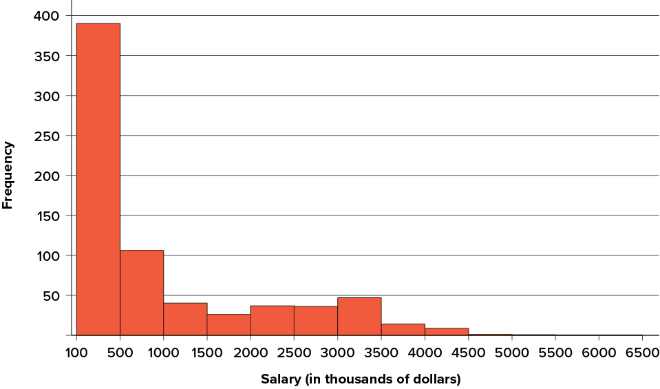
Table 3.7 shows the measures of central tendency for these data. The large skew results in very different values for these measures. No single measure of central tendency is sufficient for data such as these. If you were asked the very general question: “So, what do baseball players make?” and answered with the mean of $1,183,000, you would not have told the whole story since only about one third of baseball players make that much. If you answered with the mode of $109,000 or the median of $500,000, you would not be giving any indication that some players make many millions of dollars. Fortunately, there is no need to summarize a distribution with a single number. When the various measures differ, our opinion is that you should report the mean and median. Sometimes it is worth reporting the mode as well. In the media, the median is usually reported to summarize the center of skewed distributions. You will hear about median salaries and median prices of houses sold, etc. This is better than reporting only the mean, but it would be informative to hear more statistics.
Spread and Variability
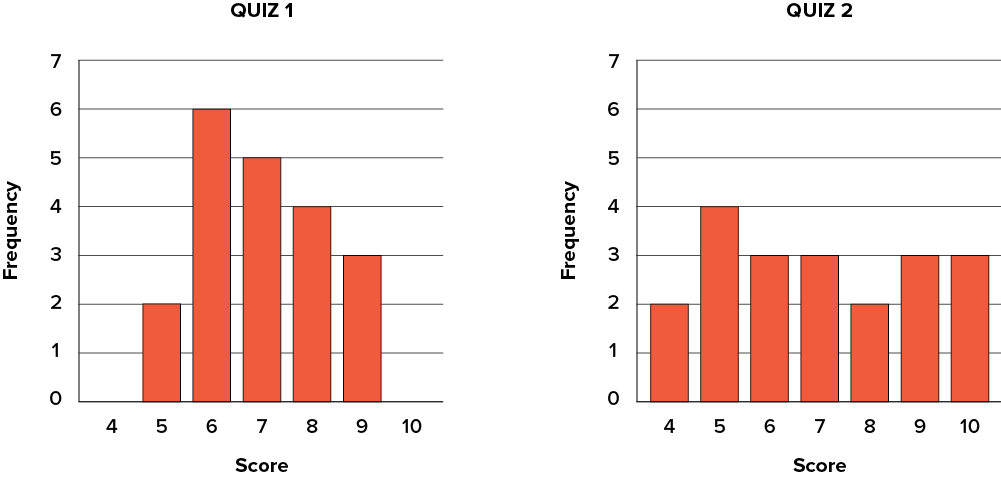
Variability refers to how “spread out” a group of scores is. To see what we mean by spread out, consider the graphs in Figure 3.10. These graphs represent the scores on two quizzes. The mean score for each quiz is 7.0. Despite the equality of means, you can see that the distributions are quite different. Specifically, the scores on Quiz 1 are more densely packed and those on Quiz 2 are more spread out. The differences among students were much greater on Quiz 2 than on Quiz 1.
Figure 3.10. Bar charts of Quizzes 1 and 2. (“Quiz Score Bar Charts” by Judy Schmitt is licensed under CC BY-NC-SA 4.0.)
The terms variability, spread, and dispersion are synonyms and refer to how spread out a distribution is. Just as in the section on central tendency where we discussed measures of the center of a distribution of scores, in this section we will discuss measures of the variability of a distribution. There are three frequently used measures of variability: range, variance, and standard deviation. In the next few paragraphs, we will look at each of these measures of variability in more detail.
Range
The range is the simplest measure of variability to calculate, and one you have probably encountered many times in your life. The range is simply the highest score minus the lowest score. Let’s take a few examples. What is the range of the following group of numbers: 10, 2, 5, 6, 7, 3, 4? Well, the highest number is 10, and the lowest number is 2, so 10 − 2 = 8. The range is 8. Let’s take another example. Here’s a dataset with 10 numbers: 99, 45, 23, 67, 45, 91, 82, 78, 62, 51. What is the range? The highest number is 99 and the lowest number is 23, so 99 − 23 = 76; the range is 76. Now consider the two quizzes shown in Figure 3.10. On Quiz 1, the lowest score is 5 and the highest score is 9. Therefore, the range is 4. The range on Quiz 2 was larger: the lowest score was 4 and the highest score was 10. Therefore the range is 6.
The problem with using range is that it is extremely sensitive to outliers, and one number far away from the rest of the data will greatly alter the value of the range. For example, in the set of numbers 1, 3, 4, 4, 5, 8, and 9, the range is 8 (9 − 1). However, if we add a single person whose score is nowhere close to the rest of the scores, say, 20, the range more than doubles from 8 to 19.
Interquartile Range
The interquartile range (IQR) is the range of the middle 50% of the scores in a distribution and is sometimes used to communicate where the bulk of the data in the distribution are located. It is computed as follows:
IQR = 75th percentile − 25th percentile
For Quiz 1, the 75th percentile is 8 and the 25th percentile is 6. The interquartile range is therefore 2. For Quiz 2, which has greater spread, the 75th percentile is 9, the 25th percentile is 5, and the interquartile range is 4. Recall that in the discussion of box plots, the 75th percentile was called the upper hinge and the 25th percentile was called the lower hinge. Using this terminology, the interquartile range is referred to as the H-spread.
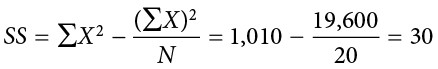
Sum of Squares
Variability can also be defined in terms of how close the scores in the distribution are to the middle of the distribution. Using the mean as the measure of the middle of the distribution, we can see how far, on average, each data point is from the center. The data from Quiz 1 are shown in Table 3.8.
There are a few things to note about how Table 3.8 is formatted. The raw data scores (X) are always placed in the left-most column. This column is then summed at the bottom (ΣX) to facilitate calculating the mean by dividing the sum of X values by the number of scores in the table (N). The mean score is 7.0 (ΣX/N = 140/20 = 7.0). Once you have the mean, you can easily work your way down the second column calculating the deviation scores ( ), representing how far each score deviates from the mean, here calculated as the score (X value) minus 7. This column is also summed and has a very important property: it will always sum to 0, or close to zero if you have rounding error due to many decimal places (Σ() = 0). This step is used as a check on your math to make sure you haven’t made a mistake. If this column sums to 0, you can move on to filling in the third column, which is composed of the squared deviation scores. The deviation scores are squared to remove negative values and appear in the third column
  . When these values are summed, you have the sum of the squared deviations, or the sum of squares (SS), calculated with the formula
 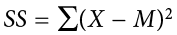 .
.
Table 3.8. Calculation of variance for Quiz 1 scores.
|
X |
X − M |
(X − M)2 |
X2 |
|
9 |
2 |
4 |
81 |
|
9 |
2 |
4 |
81 |
|
9 |
2 |
4 |
81 |
|
8 |
1 |
1 |
64 |
|
8 |
1 |
1 |
64 |
|
8 |
1 |
1 |
64 |
|
8 |
1 |
1 |
64 |
|
7 |
0 |
0 |
49 |
|
7 |
0 |
0 |
49 |
|
7 |
0 |
0 |
49 |
|
7 |
0 |
0 |
49 |
|
7 |
0 |
0 |
49 |
|
6 |
−1 |
1 |
36 |
|
6 |
−1 |
1 |
36 |
|
6 |
−1 |
1 |
36 |
|
6 |
−1 |
1 |
36 |
|
6 |
−1 |
1 |
36 |
|
6 |
−1 |
1 |
36 |
|
5 |
−2 |
4 |
25 |
|
5 |
−2 |
4 |
25 |
|
ΣX = 140
|
Σ( |
Σ |
|


The preceding formula is called the definitional formula, as it shows the logic behind the sum of squared deviations calculation. As mentioned earlier, there can be rounding errors in calculating the deviation scores. Also, when the set of scores is large, calculating the deviation scores, squaring the scores, and then summing those values can be tedious. To simplify the sum of squares calculation, the computational formula is used instead. The computational formula is as follows:
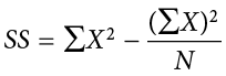
The last column in Table 3.8 represents the X values squared and then summed— . At the bottom of the first column, the
  value is squared—
 . These are the values used in the computational formula for the sum of squares. As you can see in the calculation below, the SS value is the same for both the definitional formula and the computational formula:
As we will see, the sum of squares appears again and again in different formulas—it is a very important value, and using the X and  columns in this table makes it simple to calculate the SS without error.
Variance
Now that we have the sum of squares calculated, we can use it to compute our formal measure of average distance from the mean—the variance. The variance is defined as the average squared difference of the scores from the mean. We square the deviation scores because, as we saw in the second column of Table 3.8, the sum of raw deviations is always 0, and there’s nothing we can do mathematically without changing that.
The population parameter for variance is s2 (“sigma-squared”) and is calculated as:

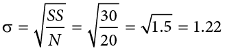
We can use the value we previously calculated for SS in the numerator, then simply divide that value by to get variance. If we assume that the values in Table 3.8 represent the full population, then we can take our value of sum of squares and divide it by to get our population variance:

So, on average, scores in this population are 1.5 squared units away from the mean. This measure of spread exhibits much more robustness (a term used by statisticians to mean resilience or resistance to outliers) than the range, so it is a much more useful value to compute. Additionally, as we will see in future chapters, variance plays a central role in inferential statistics.
The sample statistic used to estimate the variance is s2 (“s-squared”):
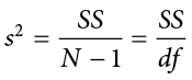
This formula is very similar to the formula for the population variance with one change: we now divide by N − 1 instead of . The value N − 1 has a special name: the degrees of freedom (abbreviated as df). You don’t need to understand in depth what degrees of freedom are (essentially they account for the fact that we have to use a sample statistic to estimate the mean [] before we estimate the variance) in order to calculate variance, but knowing that the denominator is called df provides a nice shorthand for the variance formula:

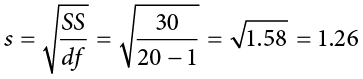
Going back to the values in Table 3.8 and treating those scores as a sample, we can estimate the sample variance as:
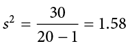
Notice that this value is slightly larger than the one we calculated when we assumed these scores were the full population. This is because our value in the denominator is slightly smaller, making the final value larger. In general, as your sample size gets bigger, the effect of subtracting 1 becomes less and less. Comparing a sample size of 10 to a sample size of 1000; 10 − 1 = 9, or 90% of the original value, whereas 1000 − 1 = 999, or 99.9% of the original value. Thus, larger sample sizes will bring the estimate of the sample variance closer to that of the population variance. This is a key idea and principle in statistics that we will see over and over again: larger sample sizes better reflect the population.
Standard Deviation
The standard deviation is simply the square root of the variance. This is a useful and interpretable statistic because taking the square root of the variance (recalling that variance is the average squared difference) puts the standard deviation back into the original units of the measure we used. Thus, when reporting descriptive statistics in a study, scientists virtually always report mean and standard deviation. Standard deviation is therefore the most commonly used measure of spread for our purposes, representing the average distance of the scores from the mean.
The population parameter for standard deviation is s (“sigma”), which, intuitively, is the square root of the variance parameter s2 (occasionally, the symbols work out nicely that way). The formula is simply the formula for variance under a square root sign:
The sample statistic follows the same conventions and is given as s in mathematical formulas. (Note that in American Psychological Association [APA] format for reporting results, sample standard deviation is reported using the abbreviation SD.)
The standard deviation is an especially useful measure of variability when the distribution is normal or approximately normal because the proportion of the distribution within a given number of standard deviations from the mean can be calculated. For example, 68% of the distribution is within one standard deviation (above and below) of the mean and approximately 95% of the distribution is within two standard deviations of the mean, as shown in Figure 3.11. Therefore, if you had a normal distribution with a mean of 50 and a standard deviation of 10, then 68% of the distribution would be between 50 − 10 = 40 and 50 + 10 = 60. Similarly, about 95% of the distribution would be between 50 − 2 × 10 = 30 and 50 + 2 × 10 = 70.
Figure 3.11. Percentages of the normal distribution. (“Normal Distribution Percentages” by Judy Schmitt is licensed under CC BY-NC-SA 4.0.)
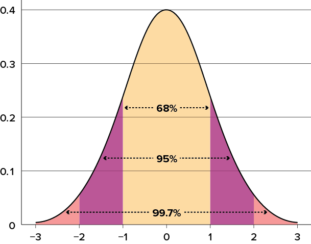
Figure 3.12 shows two normal distributions. The red (left-most) distribution has a mean of 40 and a standard deviation of 5; the blue (right-most) distribution has a mean of 60 and a standard deviation of 10. For the red distribution, 68% of the distribution is between 45 and 55; for the blue distribution, 68% is between 50 and 70. Notice that as the standard deviation gets smaller, the distribution becomes much narrower, regardless of where the center of the distribution (mean) is. Figure 3.13 presents several more examples of this effect.
Figure 3.12. Normal distributions with standard deviations of 5 and 10. (“Normal Distributions with Standard Deviations” by Judy Schmitt is licensed under CC BY-NC-SA 4.0.)
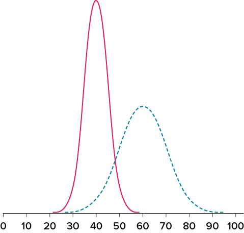
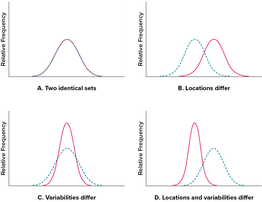
Figure 3.13. Differences between two datasets. (“Location and Variability Differences” by Judy Schmitt is licensed under CC BY-NC-SA 4.0.)
Exercises
- If the mean time to respond to a stimulus is much higher than the median time to respond, what can you say about the shape of the distribution of response times?
- Compare the mean, median, and mode in terms of their sensitivity to extreme scores.
- Your younger brother comes home one day after taking a science test. He says someone at school told him that “60% of the students in the class scored above the median test grade.” What is wrong with this statement? What if he had said “60% of the students scored above the mean?”
- Make up three datasets with five numbers each that have:
- the same mean but different standard deviations.
- the same mean but different medians.
- the same median but different means.
- Compute the population mean and population standard deviation for the following scores (remember to use the sum of squares table): 5, 7, 8, 3, 4, 4, 2, 7, 1, 6
- For the following problem, use the following scores: 5, 8, 8, 8, 7, 8, 9, 12, 8, 9, 8, 10, 7, 9, 7, 6, 9, 10, 11, 8
- Create a histogram of these data. What is the shape of this histogram?
- How do you think the three measures of central tendency will compare to each other in this dataset?
- Compute the sample mean, the median, and the mode
- Draw and label lines on your histogram for each of the above values. Do your results match your predictions?
- Compute the range, sample variance, and sample standard deviation for the following scores: 25, 36, 41, 28, 29, 32, 39, 37, 34, 34, 37, 35, 30, 36, 31, 31
- Using the same values from Problem 7, calculate the range, sample variance, and sample standard deviation, but this time include 65 in the list of values. How did each of the three values change?
- Two normal distributions have exactly the same mean, but one has a standard deviation of 20 and the other has a standard deviation of 10. How would the shapes of the two distributions compare?
- Compute the sample mean and sample standard deviation for the following scores: −8, −4, −7, −6, −8, −5, −7, −9, −2, 0
Answers to Odd-Numbered Exercises
1)
If the mean is higher, that means it is farther out into the right-hand tail of the distribution. Therefore, we know this distribution is positively skewed.
3)
The median is defined as the value with 50% of scores above it and 50% of scores below it; therefore, 60% of score cannot fall above the median. If 60% of scores fall above the mean, that would indicate that the mean has been pulled down below the value of the median, which means that the distribution is negatively skewed
5)
= 4.80, s2 = 2.36
7)
Range = 16, s2 = 18.40, s = 4.29
9)
If both distributions are normal, then they are both symmetrical, and having the same mean causes them to overlap with one another. The distribution with the standard deviation of 10 will be narrower than the other distribution.
