4 Guidelines for Image Evaluation
This chapter introduces a process for evaluating radiographic exams and introduces the four image properties essential to the accuracy and visibility of the image.
Learning Objectives
At the end of this chapter, you should be able to:
- Describe a process for evaluating the quality of radiographic images.
- List the four image properties that are used together to evaluate a radiographic image.
- Define each of the four image properties.
- Begin to recognize the four image properties on a radiograph.
- Identify the image properties that influence the accuracy of the image and those that influence the visibility of the image.
- Explain how the accuracy and visibility of the image can be separate entities.
Key Terms
Characteristics of the Optimal Image
When we create an image we must determine whether that image is sufficient to meet the needs of the radiologist before completing the study and sending the images for interpretation. Optimal images are essential to arriving at correct diagnoses, and correct diagnoses are critical to patients achieving positive health outcomes. See Figure 4-1 for the Characteristics of Optimal Images. Our patients have entrusted us with their care and we need to honor that trust by providing them with the highest quality services we can provide. The ASRT Practice Standards set the expectation that “the medical imaging professional strives to provide optimal care.” Part of the provision of optimal care involves the consistent, on-going evaluation of image quality and the creation of an action plan to address identified deficiencies in exam outcomes.
Figure 4-1: Evaluating the Quality of a Radiographic Image
The above criteria provide a guide for evaluating your radiographic images.
An optimal image is one where the legal requirements of the image are satisfied and the image properties maximize its diagnostic value. The image properties can be divided into the properties that describe the visibility of the image and those that describe the accuracy of the image. The visibility features of the image include brightness and contrast. The accuracy features of the image include spatial resolution and distortion. These features will be examined in depth below.
Key Takeaways
An optimal image is one where the legal requirements of the image are satisfied and the image properties maximize its diagnostic value.
Legal Requirements of Medical Images
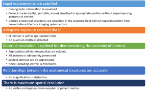
Because physicians depend on radiographs to make treatment decisions, it is essential that the information provided on the images is accurate and complete. Insuring the accuracy of this portion of the medical record is the radiographer’s responsibility. Failure to verify these details can put the radiographer, the physician and the healthcare facility at legal liability should errors in the documentation lead to a medical error. These requirements include ensuring the accuracy of the demographic information, accuracy and position of markers, and inclusion of all pertinent anatomy without artifacts or errors. See Figure 4-2.
Figure 4-2: Satisfying Legal Requirements
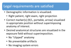
Demographics
When setting up a room for an imaging exam, the technologist will routinely select the patient from the patient worklist and open the exam(s) to be performed. While it may seem like an obvious thing, it is essential for the technologist to select the correct patient. This step links the images in the PACS system (Picture Archiving and Communications system, where patient images are stored) to the request from the ordering physician and the report from the radiologist that are stored in the hospital information system(HIS) and the radiology information system (RIS), respectively. The demographics that should be verified include the patient’s name, date of birth, and any other identifiers as required by your facility.
Patient Identity
Confirming the identity of your patient, much like verifying the drug you are administering, should be done three times: 1) when accompanying the patient from the waiting room, 2) when looking at the demographic data on the computer prior to making the first exposure, and 3) prior to completing the exam and sending it to the radiologist for interpretation. There are a variety of reasons that the patient you have in the room may not be the patient that is pulled up from the worklist – The patient could have a hearing deficit and answered to the wrong name (this is why we have them supply at least one form of identification). The technologist could have selected the wrong patient from the worklist (this happens more frequently when performing exams as a team). The exam could have been ordered on the wrong patient. You get the idea.
If a discrepancy between the patient who was imaged and the patient listed on the exam demographics is recognized before the study is sent to PACS, the technologist can easily reassociate the images with the correct patient. Once the study is sent to PACS, it becomes immediately available to an array of individuals. This incorrect information can cause the resulting diagnosis to be associated with the wrong patient and lead to unnecessary testing or treatment for the incorrect patient, and delayed interventions for the correct one. Further, if an exam is associated with the incorrect patient, once the images are sent to PACS, it becomes extremely difficult to relocate the study to make corrections. If the error is recognized after the study is sent to PACS, a PACS administrator must be notified immediately to correct the error before the images are viewed.
Ordered Exam
While you are verifying things with the patient, it is also a good idea to verify the exam that you have on the worklist is the exam the patient is expecting to have performed – both the study and the side of the body. Don’t assume that the physician made a mistake and entered the wrong side. There are good reasons to get comparison images from the non-injured side. A quick call to the ordering physician or clinic can save the patient radiation dose and a return trip to radiology. Correcting errors in the exam type and descriptors is easier before the imaging is performed, but the corrections can be made in the verbal descriptors as long as the correct projections have been obtained. The exam performed must conform to the routine protocol for the study ordered and achieve the indications for the exam provided in the clinical history. Inaccuracies in the ordered study must be corrected to reflect the correct study and indications for the exam or the radiographer may be at fault for not completing the study as ordered.
Image Projection
In addition to selecting the patient from the worklist, you will also be expected to select the projection that you are performing. This selection insures that your image is compared to the correct histogram when the computer rescales the image. If the image is processed under the wrong projection, for example your lateral chest was acquired under the PA chest designation, you can reprocess the image under the correct algorithm. You just need to know that a correction needs to be made. The PACS system also uses the image projection designation to pull the comparison images for the radiologist during interpretation. If the incorrect projection label remains associated with the image, incorrect comparison projections will be selected for the interpretation of this image and this image will be incorrectly selected for comparison to future images.
Markers
Correct identification of the orientation of the patient is vital – particularly in comparison studies, on follow-up exams and in medicolegal cases. It is essential that the radiographer use physical side markers that are clearly placed in the radiation field. These markers are made from a radiopaque material, usually lead. Because the lead absorbs the x-ray photons, the silhouette of the letters in the marker are visible as white or bright areas on the image. From a legal standpoint, markers that are embedded into the image signal ensure that the marking of the image has not been tampered with. Because digital images can be rotated and flipped and annotated labels can be applied to the image at any time, the annotated labels may be less reliable. Since annotated labels are applied to the image after exposure, their use can call into question whether the current label is the same label that was on the image at the time of radiologist’s reading or other medical decision-making, or if the label has been altered to “cover up” errors. The side marker is the most critical one to have embedded in the radiation field. Other markers may be used to indicate “side up” on decubitus images, or projections that were performed with the patient “upright,” “weight bearing” on the part, or “prone.” Markers may also be used to indicate time progression of the exam, and include options like “Scout,” “Prelim,” “Post Void,” “Post Evac,” “Post Reduction,” or time in minutes. These optional markers communicate important information to the radiologist and validate that the projections requested by the referring physician or departmental protocols have been followed. Because these markers contain more characters, it may be more desirable to annotate these labels rather than applying them to the image receptor to avoid obscuring the anatomy of interest. See Figure 4-3 for examples of embedded markers and annotated labels.
Figure 4-3: Embedded Markers vs. Annotated Labels
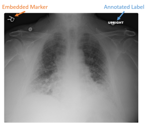
Embedding the outline of lead side markers into the radiation signal assures the viewer that the marker was in position during the creation of the image. It is impossible to determine when annotated labels were applied to the image. This calls the existence of that information during the medical decision-making process into question.
Marker Placement
Side markers should be placed directly on the image receptor or table top, just inside the collimated border. It is poor form to place the marker on the patient’s body. This practice distorts the shape of the marker, increases the risk of projecting the marker off the image (See Figure 4-4) and can spread disease-causing microorganisms.
Figure 4-4: Markers Distorted or Projected Off the Image
When markers are placed on the patient’s body, the added distance can cause the image of the marker to be projected off the image receptor. The angle of the marker placed on the patient’s abdomen, as seen in the radiograph above, can cause the marker to be distorted to the point of becoming unreadable.
The location chosen should avoid areas where there is a high risk of superimposing relevant anatomy. The marker should always be placed to the lateral side of the part you are marking. On AP/PA extremity projections, while the opposite side is not typically included on the image, marking to the medial side of the part can cause confusion. For example, when imaging a left knee, if you place the left marker on the medial side of the knee, you are technically marking the right side of the left knee, not the left side. By always placing the marker laterally, you avoid these issues. For lateral extremity images, you can place the marker anywhere within the collimated field. On AP/PA projections of the torso, place the marker laterally on the side being identified at a level that is least likely to superimpose relevant anatomy. For lateral and oblique projections of the torso, you always mark the side closest to the image receptor. This means left laterals are marked “Left” and right posterior obliques are marked “Right.” There is no standard placement for markers on lateral torso images. However, when performing lateral images of the chest or spine, placing the marker anteriorly may prevent it from becoming “burnt out” and not easily visible on the image.
All Anatomy Demonstrated
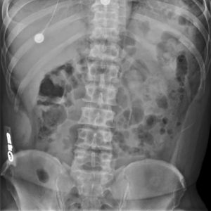
Overall, you must determine if all of the pertinent anatomy is included on the image and if there is anything present on the images that covers or obscures the anatomy. The anatomy that must be included in the exam varies from study to study, and can change depending on how the exam is being performed. Which anatomy is important for each study is a major focus of procedures courses and is essential knowledge for the radiographer. For example, a supine abdominal image must include the symphysis pubis, while an abdominal image performed upright must include the diaphragms. The variation in essential anatomy is linked to the reason for the exam. When performing abdominal imaging supine, the question the referring physician wants to answer typically is related to the intestines, but may include questions about the kidneys, ureters or bladder. Including the symphysis pubis insures that all of the bladder is included in the image. When performing an abdominal image upright, the referring physician typically is concerned with a bowel perforation or free air in the abdominal cavity. Because air rises to the highest point in the abdomen, it will collect under the diaphragms. So, in order to screen for free air, the diaphragms must be included on the image. All images where anatomy of interest is “clipped” or not included in the image must be repeated. See Figure 4-5 for an example of a portable chest x-ray where the left costophrenic angle has been clipped.
Figure 4-5: No Clipped Anatomy!
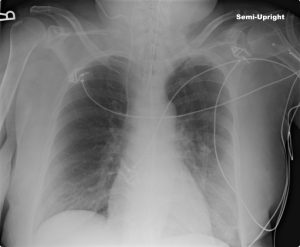
While obtaining high-quality images in a portable environment can be challenging, clipped anatomy is always a repeatable error.
No Artifacts
Artifacts are unintended structures, substances or irregularities recorded in the image that are not caused by the differential absorption of anatomic tissue. While some artifacts may be produced during image processing, most artifacts occur during the exposure of the image receptor. Prior to making an exposure, it is essential to eliminate anything from the imaging area that might cover up part of the anatomy of interest or create patterns that could mimic pathology on the image. This includes removing clothing, jewelry, glasses, hearing aids and anything else that could show up on the image. Having a patient change into a hospital gown or asking them about belongings that are near the area being imaged takes less time than repeating images once artifacts are identified. In addition to covering up anatomy of interest or mimicking pathology, artifacts can also alter the image histogram resulting in incorrect brightness and contrast of the anatomical structures on the display image. Images that contain artifacts do not need to be repeated if the artifact is outside the anatomy of interest. See examples in Figure 4-6.
Figure 4-6: Artifacts
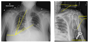
Some artifacts, like the ECG monitor wires seen on this chest x-ray, can be minimized if a little care is taken to straighten them and pull them away from the anatomy of interest. At other times, the patient’s condition necessitates that the offending objects remain in the field of view. The patient in this shoulder image was in a motor vehicle accident and the images were taken while the patient was still strapped to the backboard and in a cervical immobilization collar. Repeat images of this shoulder (which does exhibit a compression fracture of the head of the humerus) we likely necessary after the patient was removed from the backboard to fully evaluate the extent of the humerus fracture.
Image Properties
As introduced above, there are four visually significant properties of a radiographic image. These properties must blend to produce a high-quality radiographic image. Image quality refers to the faithfulness with which anatomical structures and tissues being examined are represented in the radiograph. If the anatomical part and its component tissues have sufficient visibility and accuracy to be of diagnostic value, we describe this image as a high-quality radiograph. See Figure 4-7. On one end of the spectrum are the image properties that impact the visibility of the image, and on the other end of the scale are the image properties that impact the accuracy of the image. Radiographers have to be careful not to tip the scale in favor of one property over another or they will not have a high-quality radiograph.
Figure 4-7: Image Properties
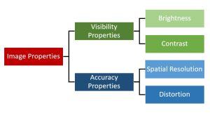
Radiographic image properties.
Image Visibility Properties
The image properties on one end of the imaging scale are those that affect the visibility of the image features. These properties are brightness and contrast. To achieve optimal brightness and contrast, we must also consider image receptor exposure and the penetration of the part.
Image Accuracy Properties
The properties on the other end of the imaging scale are those that affect accuracy of the image. These properties are recorded detail and distortion. The factors that affect these two properties are primarily related to the relationships between the body part, tube and image receptor.
Exercise 1A
The four image properties
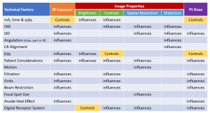
The four image properties are very important and it is necessary to understand each and the factors that control and influence them. The factors that control are considered primary factors, which means that factor should be used to change a specific image property. The factors that influence or affect are considered secondary factors, which means they usually play a more minor role in changing the image property and the radiographic quality of the image. Some of the factors can affect more than one of the four image properties. Figure 4-8 shows a table of the most important factors that control or influence image receptor exposure, the four image properties, and patient dose. A lot of these terms will be new to you. Don’t be discouraged that you don’t understand them yet. Keep referencing this important chart as you learn about the factors later on in this book. It’s good to get an overall picture first and then be able to refer back to this chart if you lose perspective.
Figure 4-8: Factors Controlling and Influencing IR Exposure, Image and Pt Dose
Brightness
Brightness describes the degree of luminance seen on the display monitor and refers to refers to the overall lightness (white) or darkness (black) of the image. We evaluate brightness in terms of the ENTIRE IMAGE. For optimum visibility, we want the image to have an intermediate brightness. If a radiography is too dark or too light it can be difficult to distinguish image features, leading to a loss of information. You may have noticed that while brightness is a key image feature, it is not included in the evaluation criteria for optimal images. This is because brightness is almost exclusively controlled by the rescaling process following histogram analysis. While mAs, kVp and patient characteristics may influence brightness, they only do so at extremely high or low levels.
Key Takeaways
Brightness is the overall lightness (white) or darkness (black) of the image.
- Brightness is evaluated in terms of the entire image.
- An intermediate brightness is optimal.
- Extreme brightness or darkness causes a loss of information.
- Brightness of the digital image is almost exclusively controlled by rescaling.
While the average brightness of the overall image is controlled by the histogram rescaling process, it is essential that the radiation reaches the image receptor in sufficient quantities to provide an adequate electronic signal.
Image Receptor Exposure
The evaluation of the image receptor exposure essentially boils down to the determination of over- or under-exposure. The wide exposure latitude afforded by digital imaging systems makes it very difficult to appreciate over- or under-exposure by visual cues alone. Soon after the development of digital imaging systems, it became apparent that some method of evaluating the exposure to the image receptor was needed. Methods of determining image receptor exposure were initially developed independently by the equipment manufacturers and the EI numbers, the methods of calculating them and even the names used to denote them varied widely. Because the scales and numbers used to indicate IR exposure could vary from room to room within a radiology department, confusion abounded and the need for a standardized method of quantifying the detector exposure was recognized. In 2009, in a joint effort between the International Electrotechnical Commission, the American Association of Physicists in Medicine and representatives from the manufacturers, a standardized IE number was developed. See Figure 4-9 for Criteria for Evaluating Receptor Exposure.
Figure 4-9: Criteria for Evaluating Receptor Exposure
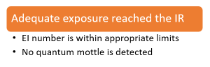
We must have an adequate number of photons reaching the image receptor or we do not have the information necessary to create the digital image.
The EI (exposure index) is defined as a measure of the amount of x-ray photons reaching the image receptor in the relative image region. The EI number is proportional to the Signal-to-Noise Ratio squared (SNR2) and related to image quality. Exposure Index calculations are calibrated by the manufacturer to ensure they are directly proportional to the image exposure. This means that when the number of photons reaching the IR is doubled by doubling the mAs, the EI number generated by the system also doubles. The EI can vary by changes in the x-ray beam quality, variations in part thickness and patient position or even variations in the voltage supplied to the x-ray tube.
Key Takeaways
To understand the definition of Exposure Index, we need to define a few more terms. The “Relevant Image Region” can be determined in two different ways. The most common method of determining the relevant image region is by equating it to the VOI obtained during histogram analysis. Histogram analysis eliminates the pixel values determined to arise from raw radiation exposure or the presence of metal or contrast media within the patient and focuses on the subject contrast arising from anatomical tissues within the patient. The average (mean) value of the pixels in the VOI is identified as the EI. An alternate method of defining the relevant image region involves calculating the average (mean) value for the pixels in the central 25% of the image receptor. This method can be problematic if the anatomy of interest is not centered over the central portion of the IR.
Key Takeaways
The Relevant Image Region can be determined in 2 ways:
- Histogram Analysis – the average value of the pixels in the VOI is used to determine the EI.
- Pixel Value of Interest – the average value of the pixels in the central 25% of the IR is used to determine the EI.
Another key term of importance is Signal-to-Noise Ratio. The Signal-to-Noise Ratio (SNR) is a measure of the efficiency and accuracy with which a digital detector captures the incident exposure and converts it to an output signal, and is controlled by the detective quantum efficiency (DQE) of the receptor system. The SNR compares incoming information (the radiation that represents the patient’s anatomy) to the level of random background information (noise). Noise, especially quantum noise, ultimately limits our ability to see an object’s edge (signal difference). Quantum mottle is a visible speckling or graininess of the image and occurs when too few photons hit the image receptor and the computer tries to fill in the missing information. See Figure 4-10 below for an example of quantum mottle on a radiographic image. Images created using a high dose (overexposed) will have a high SNR and low noise. Conversely, images created using a low dose (underexposed) will have a low SNR and high noise (quantum mottle). It can seem like increasing exposure to ensure a high SNR would be a preferred approach to selecting technical factors, however increased receptor exposure necessitates increased patient exposure and violates principles of ALARA.
Figure 4-10: Quantum Mottle
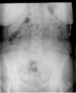
Signal-to-Noise Ratio is the percentage or ratio of useful information, i.e. signal, to non-useful or destructive information, i.e. noise, contained within an image. Images with low SNR will have high noise and exhibit a property known as quantum mottle, seen in the image above.
To be useful in the evaluation of our images, we must have a reference for our EI values. Once the EI number for the current image is determined, it must be compared to an optimum exposure value – the Target Index (EIT) – to provide actionable information. The Target Index (EIT) is the expected value of the exposure index when the image receptor is exposed properly. The EIT is specific to the detector system, projection and exam type. The EIT value must be set by the individual facility to ensure optimization of the dose to the patient without compromising the image quality. EIT does not come calibrated by the manufacturer. This can pose challenges because there is currently no standardized method for establishing the EIT.
Key Takeaways
The number quantifying the degree of variation of the actual EI from the EIT for a particular projection within a study is the Deviation Index (DI). Because the DI gives the technologist feedback on the image receptor exposure relative to an ideal exposure, the DI is more clinically valuable than the EI value. DI is a logarithmic value based on a comparison between the current EI value and the Target EI value. Once the logarithmic value is determined, it is multiplied by 10 to produce whole numbers. DI values range from below -3 to above +3, with 0 indicating that an optimum exposure was achieved.
Key Takeaways
The Deviation Index is used to provide the feedback to the technologist in the form of a color display, where the green indicates an appropriate exposure, yellow indicates a marginal exposure and red indicates a severe over- or under-exposure of the image. See Figure 4-11. In terms of DI values, positive DI values indicate overexposure, while negative DI values indicate underexposure. DI values between -1 and +1 are considered optimal, where -1 indicates an underexposure of 20% and +1 indicates and overexposure of 26%. Because of the impact that decreasing SNR has on the visibility of image features, underexposure is more detrimental to image quality than overexposure. This is seen in the ranges defining marginal exposures and gross over- and under-exposures. A DI of -3 indicates an exposure that is 1/2 the optimum exposure for the projection, while a DI of +3 indicates an exposure that is double the optimum exposure value.
Figure 4-11: Deviation Index
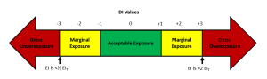
Excessive over- or under-exposure should be avoided. A DI value of -3 indicates that the exposure to the IR was less than 1/2 the optimal exposure. A DI value of +3 indicates that the exposure to the IR was 2 times the optimal exposure. While gross over- and under-exposures are to be avoided if at all possible, images should not be repeated unless the image is too noisy to distinguish relevant anatomy, or relevant anatomy is clipped or burned out.
Remember that only 1% of the radiation from the tube actually reaches the image receptor, so the EI does not reflect the patient’s exposure. The patient’s exposure will always be higher.
Key Takeaways
Contrast
In terms of visibility, it is the differences between one shade of gray in the image and another that enable the image details to be seen. We refer to these differences as contrast or radiographic contrast. Specifically, contrast is the difference between brightness levels of two or more areas of the radiograph and refers to the total number of black, white and gray tones that appear on the radiograph. It is the radiographic contrast that makes the subject contrast visible.
We evaluate contrast in terms of REGIONS within the image. Sometimes we talk about contrast in terms of contrast resolution. Resolution is the ability to image two separate objects and visually distinguish one from the other. So, contrast resolution is the ability to distinguish between differences in image intensity for structures with similar subject contrast. Contrast can be influenced by detector properties like the sensitivity to small changes in radiation exposure. See Figure 4-12 for the criteria used to evaluate an image for adequate image contrast.
Figure 4-12: Criteria for Evaluating Image Contrast
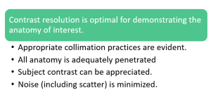
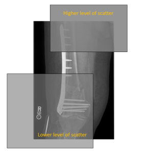
kVp will control the adequacy of beam penetration and the degree of visibility of subject contrast. Contrast resolution is also significantly influenced by the presence or absence of scatter in the image. Things that reduce the production of scatter, like using adequate collimation, will increase contrast resolution. Things that increase scatter, like the thickness of the part, will reduce contrast.
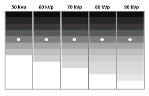
Contrast is controlled by the energy of the x-rays in the X-ray beam (i.e. the kVp you set). If you select a low kVp, the primary beam will have low energy. When the beam has lower energy, more photons will get absorbed in the patient tissues creating bigger contrast differences between the tissues. If you select a high kVp, the primary beam will have higher energy. When the beam has higher energy, more photons are transmitted through all the tissue, making the differences between the tissues smaller. The impact of kVp on contrast is demonstrated with exposures of a penetrometer or step-wedge in Figure 4-13.
We can think about contrast in terms of the size of the difference between two shades of gray. We can measure the amount of luminance of 2 adjacent steps of the step-wedge and subtract those values to obtain a mathematical representation of contrast. Images with a big difference between two adjacent shades of gray exhibit high contrast. Images with very small differences between two adjacent shades of gray exhibit low contrast.
Figure 4-13: Scales of Contrast
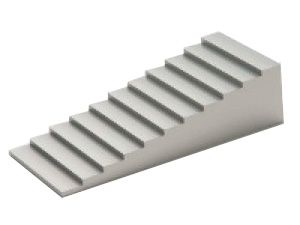
When exposures are made of an aluminum step-wedge (seen left), also known as a penetrometer, the photons of higher energies penetrate more thicknesses of aluminum or “steps.” The thinnest steps are penetrated by almost all of the energies of x-rays, while the thickest steps block nearly all energies of x-rays. The number of steps that can be seen demonstrate the scale of contrast at that energy level.
We can also think about contrast in terms of the number of shades of gray appearing in the image. Images that have very few shades of gray between black and white are said to have a short scale of contrast. If an image contains lots of different shades of gray between black and white, the image has a long scale of contrast. A radiograph that has very high contrast will appear too black-and-white. A radiograph that has very low contrast will appear too gray. For optimum visibility, we want the image to have an intermediate contrast. If the radiographic contrast is too high or too low it can be difficult to distinguish image features, leading to a loss of information. Figure 4-13 demonstrates the scale of contrast produced by radiographic exposures of a step-wedge at different kVp settings.
Key Takeaways
Contrast is defined as the total number of shades of gray visible in an image.
- Images with a short scale of contrast exhibit high contrast.
- Images with a long scale of contrast exhibit low contrast.
- An intermediate contrast is optimal.
- Extremely high or low contrast causes a loss of information.
In addition to being controlled by kVp, the contrast resolution is also influenced by the things that increase or decrease the amount of Compton scatter reaching the image. The various degrees of photoelectric absorption that occur within the anatomy create the subject contrast that forms the basis of the contrast seen on the image. Scatter radiation does not represent anatomy and coats the radiographic image in a fairly uniform layer of signal that serves to mask the contrast created by photoelectric absorption. See Figure 4-14 for a comparison of photoelectric and Compton effects on contrast. Scatter is one type of noise that degrades the visibility of the image. Quantum mottle, another type of noise that arises from inadequate receptor exposure, likewise reduces contrast and degrades the visibility of the image.
Figure 4-14: The Impact of Photoelectric and Compton Scatter on Contrast
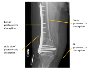
Photoelectric interactions (seen left) increase contrast. Compton Scatter (seen right), which coats the image in a uniform layer of radiation that does not represent the anatomy, decreases contrast.
While we learned in the last chapter that digital imaging systems control the total possible shades of gray with bit depth, the human visual system is only capable of discerning about 30 different shades of gray at one time. The post-processing application of changing the window width and the window level allows us to change the tissues that are highlighted in the visible range.
Key Takeaways
Contrast is also defined as the difference between brightness levels of different areas of the radiograph.
- Contrast is evaluated through a comparison of image regions.
- Contrast is primarily controlled by the kVp used in the exposure.
- Contrast is influenced by noise arising from Compton scatter or quantum mottle.
Optimal contrast resolution allows us to differentiate between small differences in tissue attenuation.
Accuracy Properties
Each radiographic projection is developed to demonstrate the anatomical relationships between structures that can most effectively support diagnosis. It is critical that each projection demonstrate the anatomy accurately. At a minimum, two images of each body part should be obtained. Those images should be taken with the central rays at right angles to each other. The process of including 2 projections at right angles to each other is termed orthogonal views. Because of the projectional nature of radiographic imaging, some anatomical structures are always superimposed with something else. By obtaining at least 2 views, we add a depth dimension that was missing from the first projection. When evaluating the accuracy of our images, we need to consider both the clarity or structural sharpness of the image and the way the size and shape of the part are demonstrated.
Spatial Resolution/Recorded Detail
As we introduced in the section on contrast, resolution is the ability to image two separate objects and visually distinguish one from the other. Spatial resolution is the ability to see two adjacent objects with high subject contrast as separate and distinct; or the ability to resolve fine details present in an object. It is sometimes referred to as recorded detail. While spatial resolution is sometimes more focused on aspects of recorded detail controlled by the image receptor and post-processing algorithms, these two terms can be used interchangeably. We evaluate spatial resolution in terms of sharpness by examining the edges of structures and the fine details, like bony trabeculation and lung markings. A radiograph that appears very sharp or clear has good spatial resolution. A radiograph that appears blurry has a poor spatial resolution. See Figure 4- 15 for criteria for the evaluation of spatial resolution.
Figure 4-15: Criteria for the Evaluation of Spatial Resolution
Anything that blurs the detail of the image decreases the accuracy of the image. This can be geometric factors or patient motion.
We measure spatial resolution in terms of line-pairs per millimeter (LP/mm).
Key Takeaways
Spatial resolution or Recorded detail is the ability to resolve fine details present in an object; or the ability to see two adjacent objects with high subject contrast as separate and distinct.
- Spatial resolution is evaluated in terms of the sharpness of the fine details in the image.
- Spatial resolution is measured in line pairs/mm, the unit of spatial frequency.
- High spatial resolution, as indicated by higher line pairs/mm, is optimal.
- Decreased spatial resolution causes a loss of information.
The unsharpness seen in an image arises from three different sources: 1) imaging system unsharpness, which is connected to the DEL size, pixel size, pixel pitch and sampling frequency used in the capture and creation of the image, 2) geometric unsharpness, which is influenced by the focal spot size, SID and OID used during the exposure, and 3) motion unsharpness, which may be voluntary or involuntary on the part of the patient, or caused by vibration or other motion of the imaging equipment.
We have seen in Ch. 3 that a larger matrix size and smaller pixel size will result in greater spatial resolution. However, the receptor matrix cannot increase spatial resolution beyond the level of detail contained in the image signal. To control the levels of recorded detail within the image signal we need to consider our radiographic distances, our selection of the focal spot size, and the risk of patient or image receptor motion.
Spatial resolution is impacted by the distances between the X-ray tube, patient and image receptor. Placing the area of interest as close to the image receptor as possible increases spatial resolution. As the OID is increased the sharpness seen within the image decreases. The opposite is true of the SID. Increasing the SID results in increased spatial resolution, while reducing the SID will decrease spatial resolution. Because of this inverse relationship, changing the SID can compensate when using a shorter OID is not possible. For example, the lateral projection of the cervical spine will always have a long OID because the shoulder prevents us from placing the patient’s neck any closer to the image receptor. When we increase the SID from 40 to 72, we compensate for the reduced spatial resolution caused by the long OID.
Poor spatial resolution can also be impacted by the selected focal spot size. Ideally, all of the x-rays used in the creation of an image would emerge from exactly the same spot – we refer to this concept as a point source. When the photons arise from a point source, only a single the “shadow” of the radiopaque object is cast. That shadow becomes our radiographic image. But having all the x-rays emitted from the same spot isn’t practical because we would melt holes in the anode. So we spread out the electrons a little. When the large focal spot is selected, the x-rays are produced in a bigger area of the anode target. This larger space where the x-rays are emitted from produces increased unsharpness of the image.
Finally, spatial resolution will result if the patient or image receptor move during the exposure. This is why we stress the importance of clear patient instructions and the use of positioning aids. When the patient understands the need to remain still during the exposure and we provide adequate support to help them maintain the part position, increased spatial resolution will result. There will be times when the patient movement is involuntary or the patient is too young or incapacitated to follow instructions. In these cases, decreasing the exposure time can reduce the risk of motion on the images. Keep in mind that decreasing exposure time requires you to increase mA to maintain receptor exposure.
Key Takeaways
Unsharpness in the details of an image occur because of:
- The image capture and display system – bigger pixels and smaller matrix sizes = lower spatial resolution
- The geometry of the projection – Longer OID, Shorter SID and Larger Focal Spot Size = lower spatial resolution
- Motion during the exposure – More motion =lower spatial resolution
Distortion
The anatomical relationships can also be altered or distorted if the relationship between the central ray and the examined part is not considered. An altered relationship between the part and the image receptor can also result in a distorted image. Distortion is the misrepresentation of the size or shape of the anatomical structures. We want to minimize distortion to ensure the accuracy of the image.
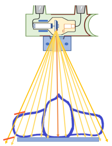
Distortion is controlled by both the distance between the X-ray tube, patient and image receptor and the alignment of the X-ray tube, patient and image receptor. When the image on the radiograph looks much bigger than the real object, the image is distorted. This type of distortion is called magnification or size distortion. When we are using photons from the center of the beam that do not diverge as much as photons further from the central ray, we see less magnification. Decreasing the SID requires us to open the collimators wider in order to cover the same area of the image receptor. Increasing the size of the collimated area includes more divergent photons in the beam and leads to greater magnification.
When the image on the radiograph looks out of shape compared with the actual object, the image is also distorted. The image may appear to be stretched out as when you pull on a piece of taffy, or it may appear squished together as when you look at yourself in a fun house mirror at an amusement park. This type of distortion is called shape distortion.
Key Takeaways
Accuracy vs. Visibility
The balance of accuracy and visibility can seem confusing at first. It’s difficult to understand how an accurate image can be produced but we might not be able to see it well. It’s also difficult to understand how we can see the image well, but at the same time it might not appear sharp or even look like the object we are trying to make an image of. A radiographic image may be accurate but not visible, and it may be visible, but not accurate.
Imagine this. Think of driving to the hospital on a foggy day. You always drive past a very pretty house that sits back from the road on a hill. Only today, you can’t see the house because of the fog. You know the house is still there, and when the fog lifts you will be able to see it again. On a radiograph, the image like the house can be recorded by the image receptor, but it may not be visible due to various conditions like too much exposure.
Now, imagine riding past the same house, but this time you are on your way home after an appointment with the eye doctor. The doctor put drops in your eyes and your vision is still slightly blurred. When you look at the house it appears blurry. You know it isn’t really blurry, and that tomorrow you will be able to see it clearly again. On the radiograph, the image may not be recorded sharply, but it is still visible.
Good Images and Bad Images
When a radiograph is produced with too little brightness, it appears too dark or black and the body parts in the image are not visible. The image of the body is still there under the darkness, and if some of the darkness is removed, the image of the body parts will be visible again. If too much darkness is removed, the image will become too light or white to see the patient’s anatomy. Figure 4-3 shows a radiograph with good brightness, one that is too dark and one that is too bright.
Figure 4-3: Comparing Brightness
A. 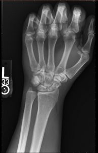 B.
B. 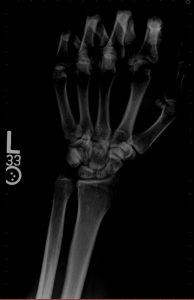 C.
C. 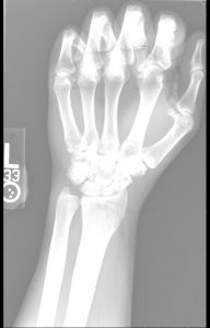
A. Radiograph with good brightness. B. Radiography that is too dark. C. Radiograph that is too bright.
When a radiograph is produced with a contrast that is too high or too low, certain parts of the image are emphasized and other parts are de-emphasized. All the parts are still there, but it is impossible to see them all at the same time on the image. Figure 4-4 shows a radiograph with good contrast, one with a contrast that is too high and one with a contrast that is too low.
Figure 4-4: Comparing Contrast
B.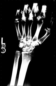 C.
C. 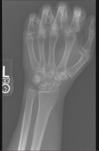
If a radiograph is produced with poor recorded detail, the image will appear blurry. The image is still there, and if it is cleared up it will be easier to see. Figure 1-4 shows a radiograph with good recorded detail and one that appears to be blurred because of motion of the patient during the exposure.
If a radiograph is produced that is distorted, the image will appear different from the actual object. The image may appear larger than the actual object or not the same shape as the actual object. This can be very confusing to the radiologist and to anybody else who looks only at the image and hasn’t seen what the real object looks like. It is the radiographer’s job to make the image look as much like the real object as possible. Figure 1-5 shows a radiograph without distortion, one with magnification or size distortion, and one with shape distortion.
Summary
There are four image properties that affect the overall quality of the finished radiograph. They are brightness, contrast, recorded detail and distortion. Brightness and contrast are visibility properties, and recorded detail and distortion are accuracy properties. A good radiographic image will have a balance of the four characteristics. There are many factors that influence these properties, and a good radiographer can manipulate the factors to produce an excellent radiograph.
Describes the degree of luminance seen on the display monitor and refers to refers to the overall lightness or darkness of the image. Brightness is one of the properties that comprise visibility of image features, and is related to the idea of window level.
The difference between brightness levels of adjacent pixels in the radiograph; the total number of shades of gray that represent the different structures on the image. Contrast is one of the properties that comprise visibility of image features, and is related to the idea of window width.
The misrepresentation of the true size or shape of the structure being examined.
The weighted combination of all of the visually significant characteristics of an image that contribute to the diagnostic value of the image.
Proportionally increasing or enlarging both axes of a structure.
Movement of the patient during the exposure; This blurs the image.
Noise is noninformational variations in pixel level that reduces the visibility of detail in the resulting image, and includes anything that hides the signal, including scatter and electronic noise. Noise may cause a grainy or uneven appearance of an image when an insufficient number of x-rays reach the image receptor (see quantum mottle).
The sharpness of the lines of the structures included in the image. Recorded detail is related to the concept of spatial resolution.
Proportionally increasing or enlarging both axes of a structure. Synonymous with Magnification.
The ability of the imaging system to resolve fine details present in an object.