6 kVp – Reorganized
As introduced in Ch. 5, the radiographer must set certain exposure factors on the control panel before each and every x-ray exposure. How these factors are set determines the finished quality of the radiograph, as well as the radiation dose to the patient, so their proper selection is very important. If the radiograph has to be repeated because the exposure factors were selected improperly, the patient gets an unnecessary extra dose of radiation.
In this chapter you are going to learn about another of the primary exposure factors: kilovoltage, and its relationship to the quality of the IR exposure, patient dose and the four image properties. You will learn about the relationship of kVp to the production of scattered radiation and how it impacts image quality. You will also learn about optimum kVp, which is the exposure factor that should be selected first by the radiographer, and how to apply the 15% Rule, which is a calculation used to balance changes in kVp with changes in mAs.
Learning Objectives
At the end of this chapter, you should be able to:
- Define kVp and explain its relationship to IR exposure, the four image properties and patient dose.
- Explain why kVp causes a heterogeneous x-ray beam.
- Describe how the photon energy, radiographic contrast and scale of contrast vary as the kVp is changed.
- Describe the production of scattered radiation and its effect on radiographic contrast.
- Explain how kVp affects the production of scattered radiation.
- Define optimum kVp.
- List the optimum kVp for commonly radiographed body parts.
- State the controlling factor for IR exposure and for contrast.
- State the relationship of mAs to IR exposure and to contrast.
- State the relationship of kVp to IR exposure and to contrast.
- Describe and calculate the 15% rule.
- Apply the 15% rule to control radiographic contrast.
- Apply the 15% rule to control motion.
- Calculate the 15% rule changes in the 60 – 90 kVp range.
Key principles of kVp
Kilovoltage (kVp) is a measure of the electrical force driving the electrons through a circuit. It is also referred to as potential difference or electromotive force. The term electromotive force paints a vivid picture of what kilovoltage does – it provides the force to move the electrons. In Ch. 1, we discussed the production of x-rays in detail. When x-rays are produced, electrons are released from the filament in the x-ray tube. These electrons are rapidly pulled across the tube to the anode, are stopped suddenly by the anode, and give up energy in the form of x-rays. The kinetic energy of the electrons is converted into x-ray energy at the anode.
If an electron has a high amount of kinetic energy, it has the potential to give up more energy at the anode than an electron with a low amount of kinetic energy. If an electron gives up a high amount of kinetic energy, it produces a photon with a high amount of energy. And if an electron gives up a low amount of energy, it produces a photon with a low amount of energy.
kVp is the factor that determines the energy of the x-ray photons produced because it determines the amount of kinetic energy each electron has as it moves from the filament to the anode. Kilovoltage is produced in the form of a wave over the time of the exposure. The “p” in kVp stands for peak. The peak voltage is the highest voltage reached during an electical cycle. The kVp that is set on the control panel is the maximum or peak kilovoltage reached during the exposure.
Key Takeaways
kVp is the unit of potential difference or electromotive force. It is the force that drives the electrons across the tube.
- The “p” in kVp stands for peak – the highest voltage reached during an electrical cycle.
- When we set kVp we are specifying the highest voltage going through the x-ray circuit.
As we saw in Ch. 4, kVp is the technical factor we use to control contrast (See Figure 6-1, below), but our kVp choices will also significantly impact IR exposure and patient dose.
Figure 6-1: kVp’s Impact on IR Exposure, Image Properties and Pt. Dose
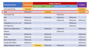
We use kVp to Control contrast, but it also significantly affects IR exposure and Patient Dose.
kVp and X-Ray Production
In Ch. 1 we learned that when the incident electrons interact with the atoms making up the anode, they can lose their kinetic energy in two ways – Characteristic interactions eject an inner shell electron and x-rays are produced with outer shell target electrons drop into the inner shell hole. Bremstrahlung interactions slow down the incident electron based on its proximity to the positively charged nucleus and an x-ray is produced that is proportional to the amount of slowing that the incident electron undergoes.
While a few incident electrons release all of their kinetic energy in a single brems interaction, most electron interactions result in the loss of less energy. In both brems and characteristic interactions, the incident electron may interact multiple times before it loses all of the kinetic energy it gains from accelerating across the x-ray tube. The number of times that the incident electron bounces around before it can calmly join the flow of electrons in the circuit is dependent on its kinetic energy. Higher energy electrons have more energy to expend and undergo more interactions than electrons with lower kinetic energy . Each interaction produces x-rays or heat.
Key Takeaways
Increasing kVp leads to greater efficiency in x-ray production, i.e. more photons produced per electron.
- Higher kVp = more target interactions = more x-rays
KVp and Photon energy
The energy of x-ray photons is measured in kiloelectron volts (keV). One electronvolt (symbol eV) is a unit of energy equal to the amount of kinetic energy gained by a single electron accelerated from rest through an electric potential difference of one volt in vacuum. Because we are accelerating electrons through a vacuum when we are making x-rays, we measure the kinetic energy gained by the electrons and the energy released as x-rays in units of electron volts. Since we are accelerating the electrons with kilovoltages, we produce x-rays with energies in kiloelectron volts. The kVp we select on the control panel will determine the maximum energy in keV of the x-rays produced. For example, when operating an x-ray machine at 80 kVp, the x-ray energies produced will range from zero to 80 keV.
Key Takeaways
The energy of an x-ray is measured in kiloelectron volts (keV).
- The kVp selected on the control panel will determine the maximum x-ray energy in electron volts.
If the radiographer selects a high kVp, most of the electrons will have a lot of kinetic energy as they move toward the anode and a large percentage of the photons produced in the x-ray beam will have a lot of energy. If the radiographer selects a low kVp, the electrons have less kinetic energy an a large percentage of the photons produced will have a low amount of energy.
Key Takeaways
- Higher kVp = more energy released = higher energy x-rays
- Lower kVp = less energy released = lower energy x-rays
kVp and The Primary Beam
Recall from Ch. 1 that we can make a graph of the number of photons that occur at the different photon energies within the primary beam. We call this graph an emission spectrum. Also recall that the characteristic interactions create discrete peaks on the graph because they have only a few specific energy levels, while bremstrahlung interactions create a continuous, bell shaped curve. The area under the curve, plus the photons represented in the characteristic spikes, represents the total number of photons in the beam. If the area under the curve increases, we have more photons in the beam. See Figure 6-2.
Figure 6-2: Emission Spectrum
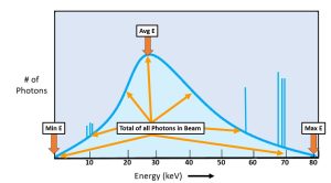
The emission spectrum is a graphic representation of the number of photons in the beam at different energy levels.
Emission spectra (-um is singular, -a is plural) are one way to compare how our technical factor changes change the quality and quantity of the beam. A change in beam quantity will shift the amplitude of the bremstrahlung curve up or down. A change in the beam quality will shift the average energy of the beam left or right.
kVp and Beam Quantity
Recall from Ch. 1 that beam quantity or intensity is the total number of photons in the primary x-ray beam. Electrons may interact multiple times before expending all of their kinetic energy. More kinetic energy results in more interactions. More interactions create more x-rays. We can see this in the emission spectra. See Figure 6-3.
Figure 6-3: kVp’s Impact on Beam Quantity
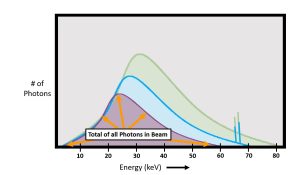
The purple graph of the photons created with 60 kVp has less area under the curve, so less total photons in the beam. Compared to the green graph of photons created with 80 kVp, which has much greater area under the curve. This means that more photons were created when we use 80 kVp than are created when we use 60 kVp.
As we increase the kVp from 60 to 70 to 80, we see that the amplitude of the curves gets progressively higher. The purple curve created by the 60 kVp beam has the fewest number of photons in the graph, so the graph is shorter than the curves for 70 and 80 kVp. The electrons that created the 60 kVp curve acquired less kinetic energy in their trip across the x-ray tube and, consequently, each electron bounced around less and made fewer x-rays than the electrons in the other two curves. The x-ray quantity is directly proportional to the kVp2. This means that doubling the kVp will result in a four times increase in photon quantity. For example, if the kVp is increased by a factor of 2, the beam intensity increases by a factor 2 squared or 4. This is why the kVp is usually changed in small increments.
Key Takeaways
The number of photons in the beam is directly proportional to the kVp2
- Higher kVp = more target interactions = more photons in the beam
- Lower kVp = fewer target interactions = fewer photons in the beam
kVp and Beam Quality
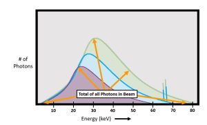
Higher energy electrons will create x-rays with a higher maximum energy. We can see these differences in the emission spectra where each curve intersects the x-axis on the right side of the graph. The non-zero x-intercept of the curve represents the highest possible photon energy in the beam. Higher kVp settings result in a non-zero x-intercept that is further to the right. See Figure 6-4.
Figure 6-4: kVp’s Impact on Beam Quality
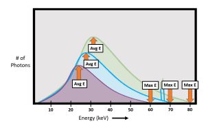
As kVp increases, both the maximum photon energy of the beam and the average energy of the beam increase.
Changes in kVp also change the average energy of the photons in the beam. The average energy of the beam is represented in the emission spectrum graph by the top of the brems “hump.” As kVp settings increase, there are more photons of higher energy in the beam. More higher energy photons increases the average energy of the beam. As kVp increases, the average energy of the beam increases and the top of the brems “hump” shifts to the right.
Key Takeaways
kVp is the primary controlling factor of beam quality.
- Increasing kVp = increased electron speed = greater photon energy
- Decreasing kVp = decreased electron speed = lower photon energy
kVp and IR Exposure
We have demonstrated above that kVp changes will change the total number of photons in the beam, but let’s consider how kVp changes impact IR exposure. The relationship between kVp and IR exposure is exponential, not linear. While the number of photons in the primary beam is proportional to the kVp squared, the relationship between IR exposure and kVp is much higher – somewhere close to kVp5. The increase in exposure at the image receptor comes from the fact that not only are there more photons in the beam, less of those photons interact inside the patient, so more photons reach the IR. However, we generally don’t want use kVp to change our IR exposure because it also changes the penetrating power of the beam and the contrast of the image.
Key Takeaways
kVp has a major impact on IR exposure, BUT shouldn’t be our first choice in changing IR exposure because it will also change the penetrating power of the beam and the contrast of the image.
- Higher kVp = more photons produced = more photons reaching the IR
PLUS
- Higher kVp = more photon energy = fewer interactions in the patient = more photons reaching the IR
Calculating the Change in IR Exposure
Because kVp can and does change the IR exposure, you may see questions about kVp’s impact on IR exposure. Because there is that exponential relationship between kVp and IR exposure, radiographers need a rule of thumb that allows us to estimate the change in IR exposure that will result from a change in kVp. That rule of thumb tells us that a 15% change in kVp will result in a change in the IR exposure by a factor of 2. So, a 15% increase in kVp will double IR exposure and a 15% decrease in kVp will cut the IR exposure in half.
To calculate an increase in 15%, multiply the original kVp by 1.15. For example, to increase 60 kVp by 15%: 60 x 1.15 = 69 kVp. To decrease the kVp using this method, you will multiply the original kVp by 0.85 (100% -15% = 85%). For example to decrease 90 kVp by 15%: 90 x 0.85 = 76.5. If rounding to the nearest whole number, 76.5 kVp will be rounded up to 77 kVp. If the answer had been 76.4 kVp, we would round down to 76 kVp.
Key Takeaways
A 15% change in kVp will result in a change in IR exposure by a factor of 2.
- Increasing kVp by 15% = 2 times (double) the IR exposure
- Decreasing kVp by 15% = 1/2 the IR exposure
kVp significantly influences IR exposure. Since kVp also changes the penetrating ability of the beam, the radiographic contrast, and the amount of scattered radiation produced, adjustment of the kVp to control IR exposure is not a good idea. Let’s make sure you understand the relationship between kVp and IR exposure.
Activity 6A – kVp and IR Exposure
The 60 to 90 kVp Range
Since most radiographers do not have calculators in their pockets at work, there is a simple way to perform most of the calculations necessary for the 15% rule. With the kVp range of 60 to 90, a 10-kVp change is equal to a 15% change.
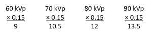
Multiply any kVp between 60 and 90 by 15% and the answer will fall between 9 and 13.5. This is close enough to the round number of 10 to make a rule of thumb. If the original kVp is between 60 and 90, add or subtract 10 kVp and either double the mAs or cut the mAs in half. These calculations can all be done easily and quickly in clinical situations.
Key Takeaways
In the 60 to 90 kVp range, a change of 10 kVp is roughly equal to a 15% change.
Using the rule of thumb to increase contrast with the original factors are 80 kVp at 7 mAs, decrease the kVp to 70 and increase the mAs to 14. Using the rule of thumb to control motion when the original factors are 80 kVp at 7 mAs, increase the kVp to 90 and decrease the mAs to 3.5 by cutting the exposure time in half.
Activity 6B – Rule of Thumb for the 15% Rule Between 60 and 90 kVp
KVP and Radiographic Contrast
While there are several exposure factors that affect radiographic contrast, kilovoltage (kVp) is the main controlling factor for radiographic contrast. This factor must be set on the control panel by the radiographer for every x-ray exposure. The kVp selected has a major influence on the quality of the radiograph.
kVp is the exposure factor that controls radiographic contrast. kVp impacts contrast in two ways – 1) by controlling the degree of absorption of photons in the beam, and 2) by changing the ratio of scatter radiation to photoelectric absorption evidenced in the image. A high kVp beam will produce a radiograph with low contrast and a low kVp beam will produce a radiograph with high contrast. A high kVp beam produces more scattered radiation than a low kVp beam. Scattered radiation reduces radiographic contrast.
Key Takeaways
kVp is the primary controlling factor of contrast.
- Higher kVp = Low Contrast
- Low kVp = High Contrast
kVp impacts contrast in 2 ways:
- Changing the differential absorption in the tissues being imaged
- Changing the ratio of scatter to photoelectric interactions seen in the image
kVp and Differential Absorption
Recall from Ch. 4 that radiographic contrast is the degree of difference between adjacent structures on a radiograph. A high contrast radiograph will appear mostly black and white with few shades of gray in between. This is called short scale contrast. A low contrast radiograph will display many shades of gray and few blacks and whites. This is called long scale contrast.
Subject contrast is caused by the composition of the patient’s body parts. Subject contrast is the number of different tissue densities and tissue thicknesses in the patient’s body. Each body tissue will display a different radiographic density depending on how x-rays passed through it and thus will contrast with each other on the radiograph. If the patient’s body parts are very similar in tissue density and thickness, contrast media can be added to the body to increase subject contrast.
Photons with low energy because of a low kVp are absorbed more easily by the atoms in the patient’s body. Differential absorption increases, and this creates an image with high contrast (short scale) which is mostly black and white. When photons have high energy, they penetrate through the body tissues more easily. The different tissues of the body are all penetrated more equally. Differential absorption decreases, and the image will have low contrast (long scale) which is many gray tones.
Key Takeaways
- More Photons Transmitted through the patient = Smaller differences in Tissue Contrast
- Smaller differences in Tissue Contrast = Low Contrast = Long Scale
The reverse is also true:
- More Photons Absorbed by the Tissues = Bigger differences in Tissue Contrast
- Bigger differences in Tissue Contrast = High Contrast = Short Scale
But more than the photon energy affects the image contrast. Contrast is also impacted by scatter radiation.
A Brief Review of Scattered Radiation
Primary radiation (radiation from the x-ray tube) enters the patient’s body and some of it is absorbed by the atoms in the body depending on the tissue density and the thickness of the body parts. The radiation that gets through the patient’s body is called exit or remnant radiation. Exit radiation hits the image receptor and is recorded as an exposure value that determines the gray level of the pixel in the displayed image. Besides exiting through the patient’s body or being absorbed by the body parts, primary radiation can also be scattered.
Scattered radiation is produced when a primary photon collides with an atom in the patient’s body, bounces off the atom, and changes its original direction. When the photon collides with the atom, it also loses some of its energy. (For a review of Compton Scattering interactions, see Ch. 2.) Since the photon has changed its direction, it could take several new paths. It could bounce directly back at the x-ray tube, it could fly out the sides of the patient’s body, or it could exit through the patient’s body and hit the image receptor from a different direction that it would have if it had remained a primary photon. It is in the patient’s body where most scattered radiation originates.
Scattered radiation that hits the image receptor puts a layer of unwanted radiation on the image that degrades the image quality. This unwanted layer of radiation is sometimes referred to as noise or fog because it appears as a blanket of grayness on the image. The fog makes the individual and distinct gray shades of the image blend in with each other sot that they cannot be seen as separate structures. The image will appear very gray and have low contrast.
Key Takeaways
Scattered radiation lowers radiographic contrast.
KVp and Scatter
Kilovoltage is the exposure factor that determines the proportion of scattered radiation reaching the image receptor. A low kVp beam has more photons with low energy and those are more easily absorbed by the atoms of the patient’s body. A photon that has already been absorbed cannot be scattered. As the energy of the photons in the x-ray beam is increased, all types of interactions within the patient’s body that attenuate the beam decrease. Overall, increasing kVp decreases the probability of the x-ray photon interacting within the patient at all, but the rate of photoelectric absorption interactions decreases faster than the rate of Compton scattering. See Figure 6-5. In this graph, we see that as photon energy increases, the total numbers of both Compton and photoelectric interactions decrease, but photoelectric interactions decrease at a much faster rate than Compton interactions do.
Figure 6-5: Number of Attenuating Interactions Compared to Photon keV
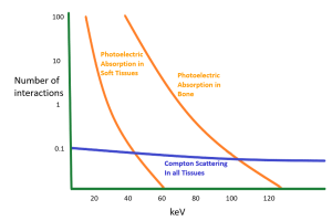
When kVp is increased, both photoelectric and Compton scattering interactions decrease, but photoelectric decreases much faster than Compton.
As the energy of photon increases, the probability of the photon interacting within the patient’s tissues decreases. However, the decrease in interactions does not occur equally. While Compton scattering makes up relatively few of the interactions at low energy levels, the total number of Compton interactions does not decrease much as photon energies increase. At low photon energies, photoelectric interactions far outweigh the Compton interactions, but as the photon energies increase the numbers of photoelectric interactions fall off quickly. This means that the ratio of photoelectric information in the beam compared to scattered radiation noise changes with changes in kVp.
Key Takeaways
The ratio of photoelectric interactions to Compton scatter decreases as kVp is increased.
- Low kVp = High Photoelectric Signal + Low Compton Scatter (noise)
- High kVp = Low Photoelectric Signal + Higher Compton Scatter (noise)
Let’s consider what these differences in the types of attenuation will mean for our images. At low photon energies of 60 keV or below, photoelectric interactions are occurring in soft tissues. These differences allow us to distinguish between soft tissue structures. For example, when imaging a lateral elbow at 55 kVp, it is easier to visualize the fat pads from muscle. This is important because these fat pads can fill with fluid subsequent to a traumatic injury and may be the only visible sign of an elbow fracture. However, above 60 keV, only transmitted x-rays from the beam represent the anatomy. Yet, the Compton scattering remains relatively stable. By the time we reach 80 kVp the blanket of scatter is making it very difficult to distinguish soft tissue details. On our elbow image, this means that at higher keV ranges, the Compton scattering may prevent the radiologist from visualizing the fat pads and result in the patient’s injury going undiagnosed. If we examine the photoelectric interactions in bone, we see that at 60 keV there are almost 100 times more photoelectric interactions than there are Compton interactions. By the time we reach 100 keV, the number of Compton and photoelectric interactions are nearly equal, and at photon energies of above 120 keV, Compton interactions predominate.
Additionally, the increased kVp produces scattered photons with a higher energy that are more likely to escape the patient’s body and interact with the image receptor. This causes the effects of scatter radiation to be more prominant on high kVp images than it is on low kVp images. The greater percentage of Compton interactions compared to Photoelectric interactions combined with greater energy of those scattered photons creates greater noise on the resultant image. Additionally, the reduction in Photoelectric interactions decreases the radiation signal that represents the anatomy. The combination of these two factors results in lower signal-to-noise ratio and less visibility of the overall image.
Key Takeaways
- High kVp = More Scattered Radiation reaching the IR + Less Signal from Photoelectric Absorption = Low Contrast = Long Scale
- Low kVp = Less Scattered Radiation reaching the IR + More Signal from Photoelectric Absorption = High Contrast = Short Scale
- Increased kVp = Decreased SNR
kVp and Scatter in Clinical Practice
While increased kVp will result in greater scattered radiation reaching our image receptor, the increased proportion of scatter only causes signal-to-noise ratio issues when the body part being imaged creates a significant amount of scatter regardless of kVp setting. More Compton scattering will occur in parts with a thickness above 10 – 12 cm (approximately 5 inches) and when large field sizes are used. Part thickness is the primary factor determining the amount of scatter produced. However, thicker parts will also require increased kVp to adequately penetrate the part. The combination of a thick part that creates a lot of scatter and a high-kVp technique that increases the energy of the scatter produced while decreasing the proportion of photoelectric interactions can lead to the production of an image with unacceptablly low contrast.
Because of the linear response rate of digital imaging systems, the computer is capable of rescaling the data into a relatively acceptable image when as little as 1% of subject contrast is present in the image data. This means that scatter radiation production is much less of a degrading factor to our images than it had been in the past. Overall, kVp selection should be more heavily based on adequate penetration of the part and reduction of patient dose than on reducing scatter.
Key Takeaways
kVp increases the percentage of scatter in the image signal, but plays less of a role in the overall impact of scatter than part thickness and collimation field size.
- More Matter = More Scatter
- The rescaling capabilities of digital imaging systems decrease the impact of scatter on the image.
We control the contrast of our images by adjusting our kVp. A 15% change in kVp is necessary to cause a perceptible change in contrast. The relationship between kVp and contrast is inversely proportional. This means that we need to increase kVp to decrease contrast and decrease kVp to increase contrast. To increase contrast, we would decrease the kVp by 15% by multiplying the original kVp by 0.85. To decrease contrast, we want to increase the kVp by 15% by multiplying the original kVp by 1.15.
Let’s practice changing kVp to control image contrast.
Activity 6C – kVp and Contrast
kVp and Spatial Resolution and Distortion
Spatial resolution and distortion are primarly influenced by geometric relationships and are not affected by the quantity or quality of the photons in the beam. kVp doesn’t change the geometric relationships used in imaging, so it does not affect spatial resolution or distortion.
Key Takeaways
We have seen that our kVp selection will impact both the IR exposure and the image contrast, but how do we determine what kVp is best to use in our exams?
Optimum kVp
A primary consideration when the radiographer selects the exposure factors to set on the control panel is the kVp, because the kVp controls the quality of the beam and its penetrating power as well as the radiation exposure to the receptor and the patient. The kVp selected should be the optimum kVp for the body part being examined. Optimum kVp is the kVp that will be able to adequately penetrate the body part, produce sufficient radiographic contrast, produce an acceptable level of scattered radiation, and minimize exposure to the patient.
Key Takeaways
Optimum kVp will:
- Penetrate the body part
- Produce sufficient contrast
- Produce an acceptable level of scatter
- Minimize patient dose
Penetration of the Part
In order to make an acceptable radiographic image, the part must be penetrated, which means the photons in the beam must have enough energy so that some of the photons will be transmitted through the part and interact with the image receptor. Kilovoltage is the exposure factor that determines the quality of the x-ray beam. The quality of the beam is determined by the energy of the photons in the beam. Photon energy determines the penetrating power of the beam. A beam produced with a high kVp will have high average photon energy. A beam produced with low kVp will have low average photon energy. A high kVp beam will be able to penetrate through the patient’s body more easily than a low kVp beam. Figure 6-6 shows the minimum kVp that should be used for the most commonly radiographed body parts.
Figure 6-6: Minimum kVp for Penetration of Common Body Parts
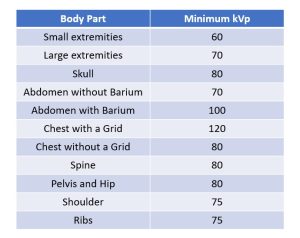
If the radiographer uses the optimum kVp, that kVp will always be able to penetrate through the body part. In general, a thick and dense body part must be penetrated with a higher kVp than a thin or less dense body part. Small extremities like hands and feet can usually be penetrated with 60 to 65 kVp, whereas at least 70 kVp is usually selected for larger extremities like the knee and elbow.
Key Takeaways
On a digital radiographic image, adequate penetration of the part can be determined by looking for evidence of quantum mottle. While quantum mottle that affects the entire image indicates inadequate photons reaching the image receptor and the need for more mAs overall, the presence of quantum mottle in the thickest portions of the patient’s anatomy and the absence of quantum mottle in thinner areas indicates the need for greater part penetration, and the need to increase kVp.
Key Takeaways
Presence of quantum mottle in only the thickest portions of the patient’s anatomy indicates the need for greater part penetration and increased kVp.
We can visualize the penetrability of our beam by using a tool called a penetrometer or step wedge. You may recall from Ch. 4 that a step wedge is a block of aluminum consisting of different thicknesses of aluminum arranged in “steps.” Lower energy photons are not able to penetrate as many steps as high energy photons. See Figure 6-8.
Figure 6-8: Using a Step Wedge to Measure Penetrability of the Beam
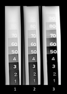
Exposure 1 was taken using 65 kVp. Exposure 2 used 75 kVp. Exposure 3 used 85 kVp.
In Figure 6-8, we can see up to the 7th step clearly in the exposure made with 65 kVp, but the steps above that are not visualized. When we increase the kVp for exposures 2 and 3, we see progressively more steps of the step wedge, demonstrating greater penetrability of the beam. You may also notice that the differences in brightness from one step to the next decrease as the penetrability increases. This demonstrates the decreased contrast that results from increased kVp settings.
Key Takeaways
The penetrating ability of the beam can be measured with a penetrometer or step wedge.
- More visible “steps” = Higher penetrability of the beam
- Fewer visible “steps” = Lower penetrability of the beam
Sufficient penetration of the part is critical to the diagnostic quality of the image. No amount of rescaling, receptor exposure or mAs can make up for information that is missing because the part was inadequately penetrated.
Sufficient Radiographic Contrast
Determination of the best radiographic contrast is somewhat subjective. A high contrast radiograph, one which appears mostly black and white with few grays, is produced with a kVp that is lower than the optimum kVp. At first glance, a high contrast radiograph may appear to be pretty and pleasing to the eye. But a closer examination of the whiter areas of the image will show that some of the anatomical parts were not demonstrated well because they were not penetrated.
A low contrast radiograph, one which is very gray, is produced with a kVp that is higher than the optimum kVp. A high kVp produces a lot of scattered radiation on the radiograph, which is what causes the very gray image. On a very gray image, it is difficult to see the separate shades of gray produced by the patient’s different body parts, so some of the patient’s anatomy may be obscured.
A radiograph with a sufficient amount of contrast, one that includes blacks, whites and an average amount of gray shades, is produced with optimum kVp. Each gray shade is seen as separate from the surrounding shades of gray. These subtle differences demonstrate anatomy that may not be seen on a high contrast or very low contrast image.
Key Takeaways
While histogram rescaling can adjust the top and bottom values of the scale of contrast for the image data, it cannot add shades of gray that do not exist in the image signal. So, an image that is captured with high contrast will remain high contrast. The computer can, however, combine exposure values to create a higher contrast image from lower contrast data. This makes a higher kVp that creates a longer scale of contrast a better option than a lower kVp that will limit the image data to a short scale of contrast.
Key Takeaways
Histogram rescaling can convert a low contrast image into one with higher contrast, but cannot create differences that were not captured in the image signal.
- Contrast needs to be balanced – not too high, not too low.
- Within the acceptable latitude of exposure values, a slightly higher kVp will prevent loss of signal information.
Scattered Radiation
The amount of scattered radiation produced in an x-ray beam is controlled by the kVp. A high kVp produces a greater percentage of scatter. Scattered radiation degrades the image by placing an extra blanked of gray noise over the image signal captured by the image receptor, which lowers radiographic contrast.
If a radiographer uses the optimum kVp for each body part, the percentage of scatter on the image remains consistent. It will vary somewhat for different patients, but it is at least predictable. Then it becomes a standard decision whether or not to use a device to control the scatter radiation.
If a radiographer used 60 kVp to radiograph an knee during one visit and on the next visit used 80 kVp, the contrast on the two radiographs would vary, the parts that were penetrated would vary, and the radiographer would need to use a grid to control scatter with the 80 kVp technique, but not with the 60 kVp technique. Thus it is better to use the optimum kVp for each body part.
Key Takeaways
kVp and Patient Dose
Changing the kVp will always change patient dose. When only kVp is changed, kVp is directly proportional to patient dose. Patient dose is directly related to the number of photons in the beam. Because beam quantity increases when kVp is increased, increasing kVp results in higher patient dose. Because beam quantity decreases when kVp is decreased, decreasing kVp results in lower patient dose. These statements assume that everything else about the exposure remains the same.
Key Takeaways
kVp controls patient dose.
- When ONLY kVp is changed, higher kVp = higher dose
The 15% Rule
We have seen that increasing kVp by 15% will double receptor exposure and decreasing the kVp by 15% will decrease receptor exposure by half. We can capitalize on this to reduce patient dose by increasing kVp within the optimum range and reducing the mAs we are using. Increasing kVp increases IR exposure by both increasing the total number of photons and the penetrating ability of those photons. mAs controls IR exposure by only changing the quantity of radiation produced. A variation in the mAs does not change the penetrating ability of the beam, the radiographic contrast or the amount of scattered radiation reaching the image receptor. mAs only controls IR exposure and does not affect contrast. We can reduce the total number of photons in the beam and still have adequate IR exposure by increasing kVp. The combination of a 15% change in kVp and a corresponding compensation by changing the mAs by a factor of 2 the 15% Rule.
The 15% Rule tells us that the IR exposure can be maintained when a 15% change in kVp is accompanied by a corresponding change in mAs. The relationship between kVp and mAs when using the 15% Rule is inverse. This means that an increase in kVp must be balanced by a decrease in mAs and decreases in kVp must be balanced by increases in mAs to maintain the same exposure to the image receptor.
If we are using the 15% Rule and compensate for increased kVp by halving the mAs, the patient’s dose will be decreased. Likewise, if we decrease kVp and double the mAs according to the 15% Rule, patient dose will be increased.
Key Takeaways
The 15% Rule tells us that IR exposure can be maintained when kVp changes are balanced with corresponding changes in mAs.
- Increased kVp + decreased mAs = same IR exposure + decreased patient dose
- Decreased kVp + increased mAs = same IR exposure + increased patient dose
- If the kVp is increased by 15%, the mAs should be cut in half.
- If the kVp is decreased by 15%, the mAs should be doubled.
Applying The 15% Rule
There are a few clinical situations when we may want to vary the mAs and optimum kVp. These instances are when the contrast needs to be changed or when the radiographer wants to help control motion of the patient.
Exposure latitude gives the radiographer room for small errors. The exposure factors can vary a little from what would be the perfect factors, and the radiograph will still be acceptable. The small range of factors cannot be exceeded or the radiograph will not be acceptable. If a radiograph taken at 10 mAs and 80 kVp is of good quality, because of exposure latitude, the mAs can be increased a little and the kVp decreased a little and the radiograph will still have acceptable IR exposure and radiographic contrast. The mAs could also be decreased and the kVp increased from the original factors and the radiograph will display the same IR exposure as the original radiograph and still be of acceptable quality.
Let’s try a couple of examples.
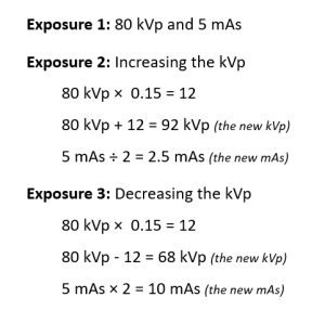
The resulting sets of exposure factors from these 3 exposures are:
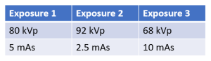
The image receptor exposure on the radiographs taken with each of these three sets of exposure factors will be approximately the same, but the contrast will be different. The radiograph from exposure 3 with the lowest kVp will have the highest contrast, while the radiograph from exposure 2 with the highest kVp will have the lowest contrast. The radiograph from exposure 1, using the optimum kVp, will have the best contrast.
Alternately, to calculate an increase in 15%, multiply the original kVp by 1.15. For example, to increase 60 kVp by 15%: 60 x 1.15 = 69 kVp. To decrease the kVp using this method, you will multiply the original kVp by 0.85 (100% -15% = 85%). For example to decrease 90 kVp by 15%: 90 x 0.85 = 76.5. If rounding to the nearest whole number, 76.5 kVp will be rounded up to 77 kVp. If the answer had been 76.4 kVp, we would round down to 76 kVp.
Activity 6D – Calculation of the 15% Rule
Using the 15% Rule to Control Contrast
The 15% rule can be applied in clinical situations to control contrast. Suppose a radiographer made an exposure of the abdomen at 80 kVp and 20 mAs. The radiograph showed adequate receptor exposure, but the contrast was too low. The contrast would be increased by using a lower kVp. In this case the mAs would have to be increased if the kVp is lowered.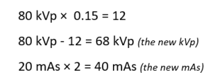
The two radiographs would have approximately the same IR exposure, but the contrast would be higher with the lower kVp.
While kVp can impact the visibility of scatter on the image, part thickness has the greatest impact on scatter production. More matter = More scatter. This places the radiographer in a somewhat difficult situation in that higher kVp levels are required to adequately penetrate thicker parts. When these thicker parts produce more scattered radiation AND that scatter has higher energy as well as outnumbering the photoelectric interactions that take place, a really ugly, low contrast image results. We cannot reduce the kVp to improve contrast or we will not penetrate the part. We have to look for other ways to decrease scatter.
There are several radiographic devices that can help control the amount of scattered radiation reaching the image receptor. The most important of those devices are the grid and the collimator. They will be discussed in Ch. 11.
Key Takeaways
Achieving a good balance between penetration, scatter and contrast can be difficult.
- First, thicker parts create more scatter. But,
- Thicker parts also need higher kVp for adequate penetration.
- High kVp and a thick part will produce a low contrast image unless other strategies to control scatter are employed.
Using the 15% Rule to Control Motion
The 15% rule can also be applied in clinical situations to control motion. Suppose a radiographer made an exposure of the skull on an uncooperative patient at 80 kVp and 20 mAs. The 20 mAs was achieved using 500 mA at 0.04 seconds. The radiograph produced was blurry as a result of motion of the patient and it need to be repeated. The radiographer would want to avoid motion on the second exposure.
Applying the 15% rule, the radiographer could increase the kVp and decrease the mAs. The decrease in mAs can be achieved by reducing the exposure time. This decrease in time would lessen the chance of having motion on the repeat radiograph. 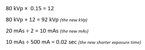
The two radiographs would have approximately the same IR exposure, but the contraast would be lower on the repeat radiograph taken with the higher kVp and shorter time. The chance of motion is less on the second exposure.
Activity 6E – 15% Rule to Control Motion and Contrast
When the 15% Rule Shouldn’t Be Used
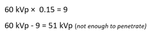
The 15% rule cannot be applied in every situation, because there are times when the range of exposure latitude would be exceeded. If the original kVp chosen is not the optimum kVp, and this kVp is at the upper or lower end of the acceptable range, a further adjustment of the kVp using the 15% rule will place the kVp above or below the acceptable range. A very low kVp may not be sufficient to penetrate the part, and a very high kVp may produce too much scattered radiation.
Suppose a radiographer chose 60 kVp to expose a radiograph of the skull. Since 80 kVp is the optimum kVp for skull radiography, the radiograph may be acceptable with 60 kVp because of exposure latitude, although some parts of the skull are not well penetrated at 60 kVp. If the radiographer reduces the kVp further according to the 15% rule, the new kVp would not penetrate the skull at all.
Suppose a radiographer chose 80 kVp to penetrate an abdomen radiograph. This kVp is already above the optimum kVp of 70. If the radiographer increases the kVp further according to the 15% rule, the new kVp would produce too much scattered radiation.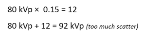
The 15% rule can only be applied over a small range of kVp changes. About 10 kVp above or below the optimum kVp is the acceptable tolerance range. A variation of more than 10 kVp will usually produce an unacceptable radiograph.
Summary
mAs controls IR exposure and kVp controls contrast. kVp influences IR exposure, but mAs does not influence contrast.
The optimum kVp should be used most of the time because it will always be enough to penetrate the body part, it will produce a sufficient level of contrast, and it will produce an acceptable amount of scattered radiation.
The 15% rule can be applied to control motion or change contrast. If the kVp is increased by 15%, the mAs can be cut in half by reducing the exposure time. This will help control motion. If the kVp is reduced by 15%, the mAs must be doubled. This will increase contrast because a lower kVp is used.
For faster calculation within the commonly used 60 to 90 kVp range, a change of 10 kVp is equal to a 15% change.
Decide which word best matches the definition or completes the sentence. Then find the work in the puzzle.
- An mA of 400 and a time of 20 milliseconds equals this mAs.
- mAs has this relationship to IR exposure.
- At 80 kVp, using the Rule of Thumb for 15%, if the mAs is cut in half, the kVp should be increased by how much?
- Short scale contrast is also this type of contrast.
- An mA of 600 and a time of 1/20 equals this mAs.
- 500 mA x 0.02 = 10 mAs and 50 mA x 0.20 = 10 mAs This illustrates what law?
- At 10 mAs, if the kVp is changed from 70 to 80, what should the new mAs be?
- The exposure factor that should be changed when the IR exposure needs to be adjusted.
- The reduction in intensity as radiation passes through matter.
- This exposure factor influences IR exposure but controls contrast.
- A high mA and low time help to control this.
- A change from 80 to 90 kVp will cause contrast to _______________.
- The radiation that emerges from the x-ray tube.
- mAs controls the ___________ of photons in the x-ray beam.
- If the kVp is increased by 15% the mAs should be cut in ___________.